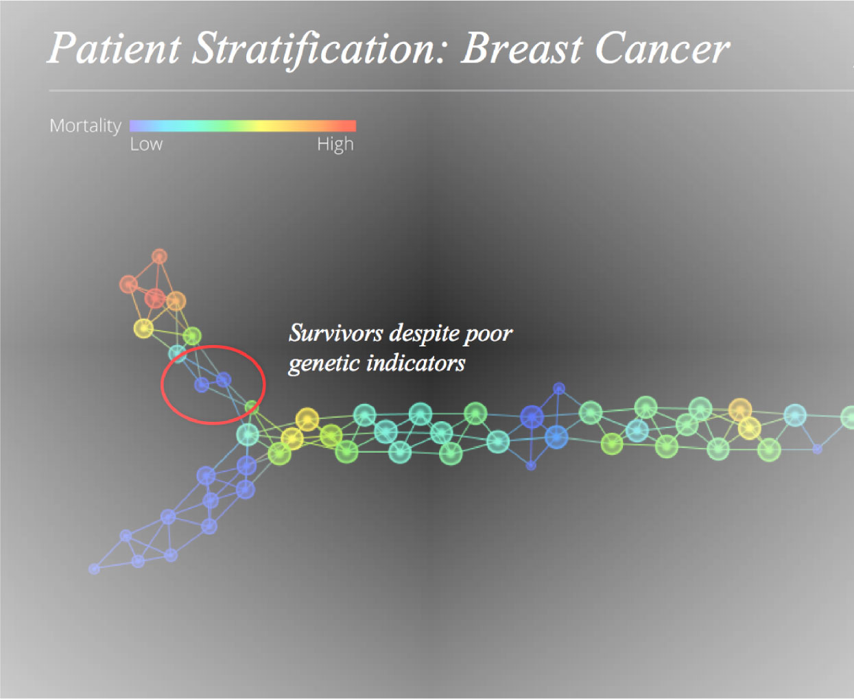
DNA microarray technology with biological data-set can monitor the expression levels of thousands of genes simultaneously. Microarray data analysis is important in phenotype classification of diseases. In this work, the computational part basically predicts the tendency towards mortality using different classification techniques by identifying features from the high dimensional dataset. We have analyzed the breast cancer transcriptional genomic data of 1554 transcripts captured over from 272 samples. This work presents effective methods for gene classification using Logistic Regression (LR), Random Forest (RF), Decision Tree (DT) and constructs a classifier with an upgraded rate of accuracy than all features together. The performance of these underlying methods are also compared with dimension reduction method, namely, Principal Component Analysis (PCA). The methods of feature reduction with RF, LR and decision tree (DT) provide better performance than PCA. It is observed that both techniques LR and RF identify TYMP, ERS1, C-MYB and TUBA1a genes. But some features corresponding to the genes such as ARID4B, DNMT3A, TOX3, RGS17 and PNLIP are uniquely pointed out by LR method which are leading to a significant role in breast cancer. The simulation is based on R-software.
Citation: Sarada Ghosh, Guruprasad Samanta, Manuel De la Sen. Feature selection and classification approaches in gene expression of breast cancer[J]. AIMS Biophysics, 2021, 8(4): 372-384. doi: 10.3934/biophy.2021029
DNA microarray technology with biological data-set can monitor the expression levels of thousands of genes simultaneously. Microarray data analysis is important in phenotype classification of diseases. In this work, the computational part basically predicts the tendency towards mortality using different classification techniques by identifying features from the high dimensional dataset. We have analyzed the breast cancer transcriptional genomic data of 1554 transcripts captured over from 272 samples. This work presents effective methods for gene classification using Logistic Regression (LR), Random Forest (RF), Decision Tree (DT) and constructs a classifier with an upgraded rate of accuracy than all features together. The performance of these underlying methods are also compared with dimension reduction method, namely, Principal Component Analysis (PCA). The methods of feature reduction with RF, LR and decision tree (DT) provide better performance than PCA. It is observed that both techniques LR and RF identify TYMP, ERS1, C-MYB and TUBA1a genes. But some features corresponding to the genes such as ARID4B, DNMT3A, TOX3, RGS17 and PNLIP are uniquely pointed out by LR method which are leading to a significant role in breast cancer. The simulation is based on R-software.

| [1] |
Ghosh S, Samanta GP (2019) Statistical modelling for cancer mortality. Lett Biomath 6: 1-12. doi: 10.30707/LiB6.1Banuelos

|
| [2] | Centers for Disease Control and Prevention, Breast Cancer in Young Women, 2020 Available from: https://www.cdc.gov/cancer/breast. |
| [3] |
Bao T, Davidson NE (2008) Gene expression profiling of breast cancer. Adv Surg 42: 249-260. doi: 10.1016/j.yasu.2008.03.002
|
| [4] | Centers for Disease Control and Prevention, Family Health History and the BRCA1 and BRCA2 genes, 2020 Available from: https://www.cdc.gov/genomics. |
| [5] |
Nicolau M, Levine AJ, Carlssonn G (2011) Topology based data analysis identifies a subgroup of breast cancers with a unique mutational profile and excellent survival. P Natl Acad Sci USA 108: 7265-7270. doi: 10.1073/pnas.1102826108
|
| [6] |
Everson TM, Lyons G, Zhang H, et al. (2015) DNA methylation loci associated with atopy and high serum IgE: a genome-wide application of recursive Random Forest feature selection. Genome Med 7: 89. doi: 10.1186/s13073-015-0213-8
|
| [7] |
Baur B, Bozdag S (2016) A feature selection algorithm to compute gene centric methylation from probe level methylation data. PLoS One 11: e0148977. doi: 10.1371/journal.pone.0148977
|
| [8] |
Mallik S, Bhadra T, Maulik U (2017) Identifying epigenetic biomarkers using maximal relevance and minimal redundancy based feature selection for multi-omics data. IEEE T Nanobiosci 16: 3-10. doi: 10.1109/TNB.2017.2650217
|
| [9] |
Breiman L (2001) Random forests. Mach Learn 45: 5-32. doi: 10.1023/A:1010933404324
|
| [10] | Ramanan D, NKI Breast Cancer Data, Data World, 2016 Available from: https://data.world/deviramanan2016/nki-breast-cancer-data. |
| [11] | Livingston F (2005) Implementation of Breiman's random forest machine learning algorithm. ECE591Q Mach Learn 1-13. |
| [12] | Gareth J, Daniela W, Trevor H, et al. (2013) An Introduction to Statistical Learning with Applications in R New York: Springer. |
| [13] | Rakotomamonjy ASupport Vector Machines and Area Under ROC curve. CiteseerX (2004) .Available from: http://citeseerx.ist.psu.edu/. |
| [14] |
Lang T, Siribaddana S (2012) Clinical trials have gone global: Is this a good thing? PLOS Med 9: e1001228. doi: 10.1371/journal.pmed.1001228
|
| [15] |
Gurdon JB, Javed K, Vodnal M, et al. (2020) Long-term association of a transcription factor with its chromatin binding site can stabilize gene expression and cell fate commitment. P Natl Acad Sci USA 117: 15075-15084. doi: 10.1073/pnas.2000467117
|
| [16] | GTR: Genetic Testing Registry, National Center for Biotechnology Information, 2009 Available from: https://www.ncbi.nlm.nih.gov. |
| [17] | Sun JW, Collins JM, Ling D, et al. (2019) Highly variable expression of ESR1 splice variants in human liver: Implication in the liver gene expression regulation and inter-person variability in drug metabolism and liver related diseases. J Mol Genet Med 13: 434. |
| [18] |
Gupta A, Hossain MM, Miller N, et al. (2016) NCOA3 coactivator is a transcriptional target of XBP1 and regulates PERK–eIF2α–ATF4 signalling in breast cancer. Oncogene 35: 5860-5871. doi: 10.1038/onc.2016.121
|
| [19] |
Quintana AM, Liu F, O'Rourke JP, et al. (2011) Identification and regulation of c-Myb target genes in MCF-7 cells. BMC Cancer 11: 30. doi: 10.1186/1471-2407-11-30
|
| [20] | Winter SF, Lukes L, Hunter KW (2010) Abstract 2371: Arid4b is a potential breast cancer progression modifier gene. Cancer Res 70: 2371. |
| [21] |
Jahangiri R, Jamialahmadi K, Gharib M, et al. (2019) Expression and clinicopathological significance of DNA methyltransferase 1, 3A and 3B in tamoxifen-treated breast cancer patients. Gene 685: 24-31. doi: 10.1016/j.gene.2018.10.060
|
| [22] | Khazayel S, Mokarram P, Mohammadi Z, et al. (2018) Derivative of stevioside; CPUK02; restores ESR1 gene methylation in MDA-MB 231. Asian Pac J Cancer P 19: 2117-2123. |
| [23] |
Li Y, Li L, Lin J, et al. (2015) Deregulation of RGS17 expression promotes breast cancer progression. J Cancer 6: 767-775. doi: 10.7150/jca.11833
|
| [24] |
Zhang G, He P, Tan H, et al. (2013) Integration of metabolomics and transcriptomics revealed a fatty acid network exerting growth inhibitory effects in human pancreatic cancer. Clin Cancer Res 19: 4983-4993. doi: 10.1158/1078-0432.CCR-13-0209
|
| [25] |
Weng T, Wang C, Hung Y, et al. (2016) Differential expression pattern of THBS1 and THBS2 in lung cancer: Clinical outcome and a systematic-analysis of microarray databases. PLoS One 11: e0161007. doi: 10.1371/journal.pone.0161007
|
| [26] | Howlader N, Noone AM, Krapcho M, et al. (2017) SEER Cancer Statistics Review, 1975–2014 Bethesda: National Cancer Institute. |
| [27] |
Kuchenbaecker KB, Hopper JL, Barnes DR, et al. (2017) Risks of breast, ovarian, and contralateral breast cancer for BRCA1 and BRCA2 mutation carriers. JAMA 317: 2402-2416. doi: 10.1001/jama.2017.7112
|
| [28] |
Weagel EG, Burrup W, Kovtun R, et al. (2018) Membrane expression of thymidine kinase 1 and potential clinical relevance in lung, breast, and colorectal malignancies. Cancer Cell Int 18: 135. doi: 10.1186/s12935-018-0633-9
|
| [29] |
Nami B, Wang Z (2018) Genetics and expression profile of the tubulin gene superfamily in breast cancer subtypes and its relation to taxane resistance. Cancers 10: 274. doi: 10.3390/cancers10080274
|
| [30] |
Marangoni E, Laurent C, Coussy F, et al. (2018) Capecitabine efficacy is correlated with TYMP and RB1 expression in PDX established from triple-negative breast cancers. Clin Cancer Res 24: 2605-2615. doi: 10.1158/1078-0432.CCR-17-3490
|
| [31] |
Ahsan H, Halpern J, Kibriya MG, et al. (2014) A genome-wide association study of early-onset breast cancer identifies PFKM as a novel breast cancer gene and supports a common genetic spectrum for breast cancer at any age. Cancer Epidemiol Biomark Prev 23: 658-669. doi: 10.1158/1055-9965.EPI-13-0340
|
| [32] |
Zancan P, Sola-Penna M, Furtado CM, et al. (2010) Differential expression of phosphofructokinase-1 isoforms correlates with the glycolytic efficiency of breast cancer cells. Mol Genet Metab 100: 372-378. doi: 10.1016/j.ymgme.2010.04.006
|
| [33] |
merc A, Sodja E, Legia M (2011) Posttranslational modification of 6-phosphofructo-1-kinase as an important feature of cancer metabolism. PloS One 6: e19645. doi: 10.1371/journal.pone.0019645
|
| [34] |
Danilova N, Kumagai A, Lin J (2010) p53 upregulation is a frequent response to deficiency of cellessential genes. PloS One 5: e15938. doi: 10.1371/journal.pone.0015938
|
| [35] |
Deng H, Yu F, Chen J, et al. (2008) Phosphorylation of Bad at Thr-201 by JNK1 promotes glycolysis through activation of phosphofructokinase-1. J Biol Chem 283: 20754-20760. doi: 10.1074/jbc.M800024200
|
| [36] |
Usenik A, Legia M (2010) Evolution of allosteric citrate binding sites on 6-phosphofructo-1-kinase. PloS One 5: e15447. doi: 10.1371/journal.pone.0015447
|
| [37] |
Landemaine T, Jackson A, Bellahcne A, et al. (2008) A six-gene signature predicting breast cancer lung metastasis. Cancer Research 68: 6092-6099. doi: 10.1158/0008-5472.CAN-08-0436
|
| [38] |
Notas G, Pelekanou V, Kampa M (2015) Tamoxifen induces a pluripotency signature in breast cancer cells and human tumors. Mol Oncol 9: 1744-1759. doi: 10.1016/j.molonc.2015.05.008
|


Figures(4) / Tables(1)

Sarada Ghosh, Guruprasad Samanta, Manuel De la Sen. Feature selection and classification approaches in gene expression of breast cancer[J]. AIMS Biophysics, 2021, 8(4): 372-384. doi: 10.3934/biophy.2021029


 DownLoad: