On slip of a viscous fluid through proximal renal tubule with linear reabsorption

Abdul M. Siddiqui; Getinet A. Gawo; Khadija Maqbool; Abdul M. Siddiqui; Getinet A. Gawo; Khadija Maqbool

doi:10.3934/biophy.2021006

AIMS Biophysics

2021, Volume 8, Issue 1: 80-102. doi: 10.3934/biophy.2021006

Previous Article Next Article

Research article Special Issues

On slip of a viscous fluid through proximal renal tubule with linear reabsorption

1.
Pennsylvania State University, 1031 Edgecomb Ave, York, PA 17403, USA
2.
Department of Mathematics and Statistics, International Islamic University, Islamabad 44000, Pakistan

Received: 05 November 2020 Accepted: 20 December 2020 Published: 05 January 2021

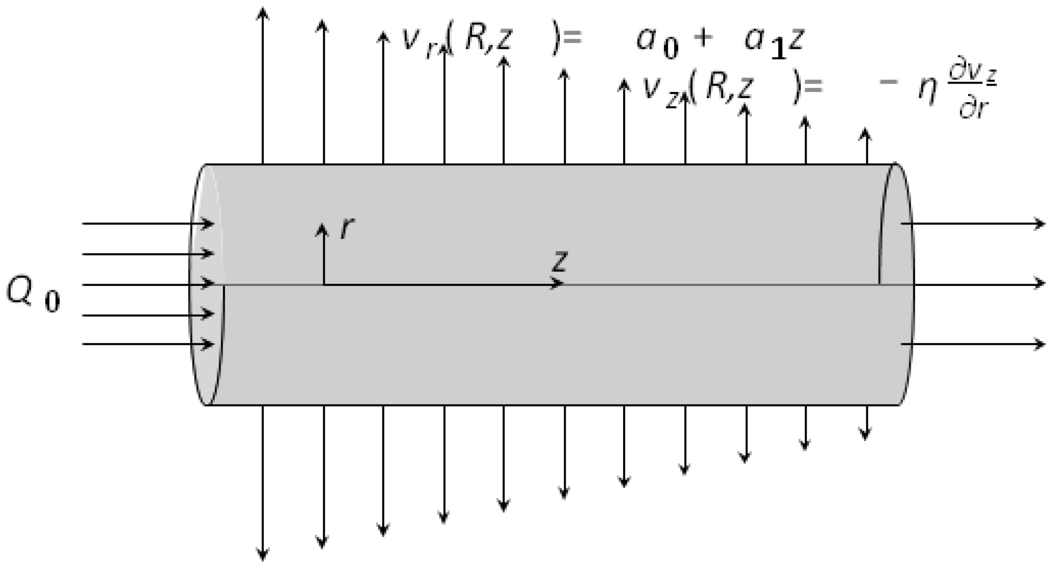
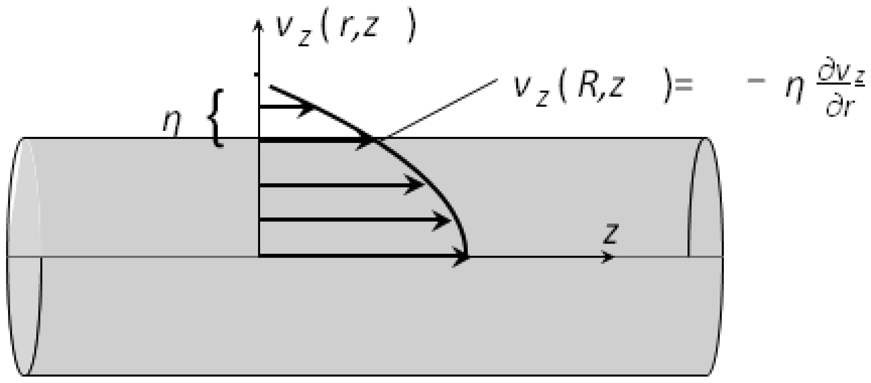
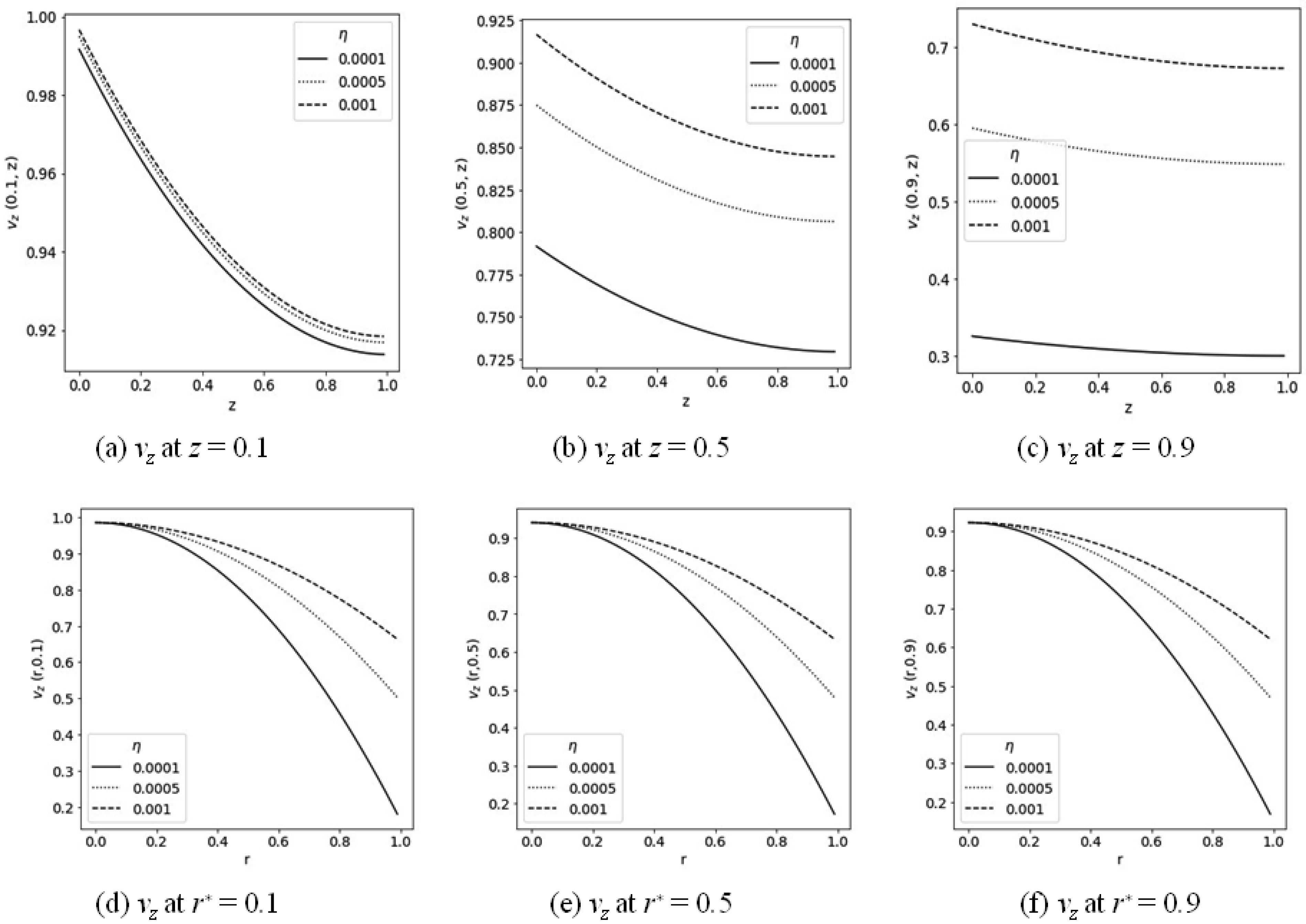
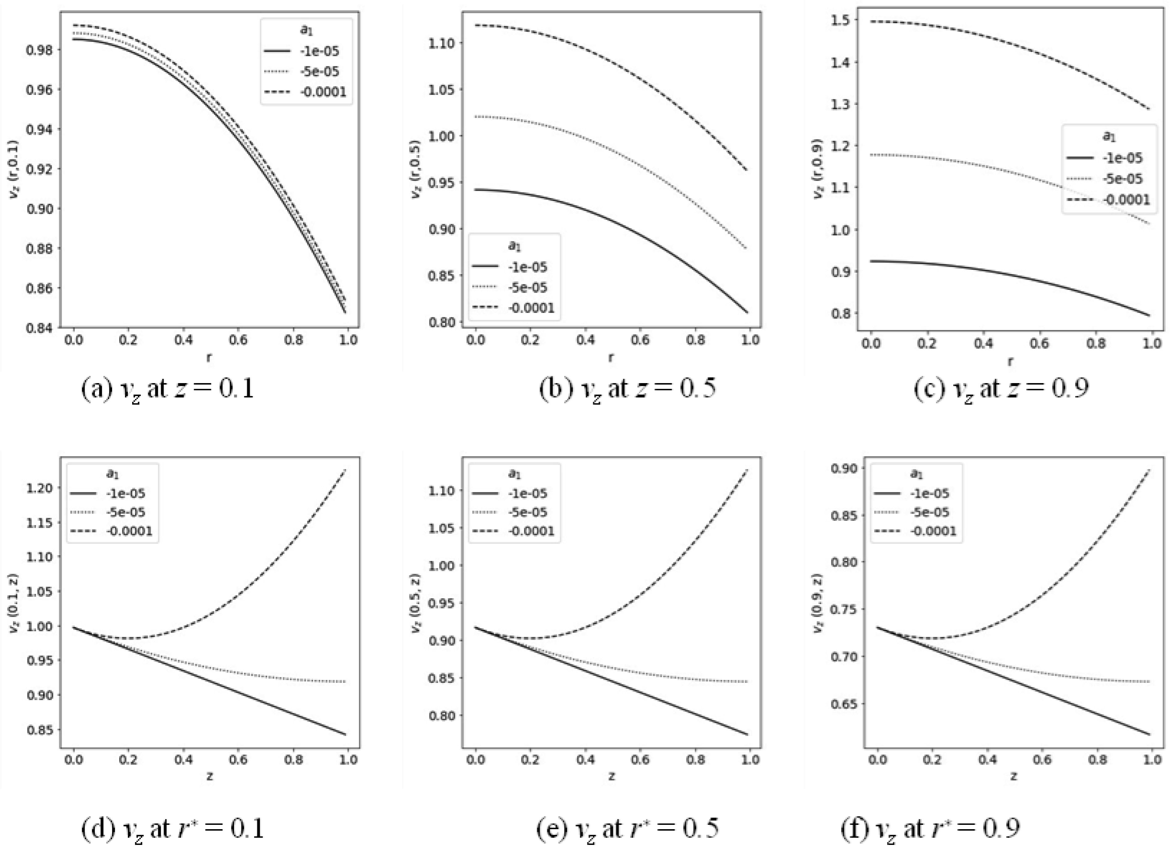
The hydrodynamical problem of flow in proximal renal tubule is investigated. Axisymmetric flow of viscous, incompressible fluid through the proximal renal tubule that undergoes linear reabsorption with slip at the wall is considered. The stream function is used to transform the governing equations to system of ordinary differential equations. The analytical solutions for velocity components, pressure distribution, fractional reabsorption and the shear stress are found. The effect of slip parameter and reabsorption rate on the flow have been investigated. The points of extreme values for the axial and radial velocity components are identified. The solution is applied to physiological data from human and rat kidney, and the results are presented in tables and graphs.
- proximal tubule,
- linear reabsorption,
- slip boundary,
- fractional reabsorption,
- flow rate
Citation: Abdul M. Siddiqui, Getinet A. Gawo, Khadija Maqbool. On slip of a viscous fluid through proximal renal tubule with linear reabsorption[J]. AIMS Biophysics, 2021, 8(1): 80-102. doi: 10.3934/biophy.2021006

Related Papers:

Abstract

The hydrodynamical problem of flow in proximal renal tubule is investigated. Axisymmetric flow of viscous, incompressible fluid through the proximal renal tubule that undergoes linear reabsorption with slip at the wall is considered. The stream function is used to transform the governing equations to system of ordinary differential equations. The analytical solutions for velocity components, pressure distribution, fractional reabsorption and the shear stress are found. The effect of slip parameter and reabsorption rate on the flow have been investigated. The points of extreme values for the axial and radial velocity components are identified. The solution is applied to physiological data from human and rat kidney, and the results are presented in tables and graphs.

Acknowledgments

Getinet Gawo would like to thank Pennsylvania State University, York Campus for the financial support provided for this work through York Campus Advisory Board Scholarly Activity Grant.

Conflict of interest

All authors have no conflict of interest.

Authors contribution

A.M Siddiqui provided the formulation of the problem, defining governing equations and boundary conditions and supervised whole paper. G. Gawo solved the governing equations and results are compared with previous works, and results are also implemented on rat kidney data. K.Maqbool revised the literature review, implemented the result on human kidney and draft the result and handled the paper submission process.

References

[1]	Macey RI (1963) Pressure flow patterns in a cylinder with reabsorbing walls. B Math Biophys 25: 1-9. doi: 10.1007/BF02477766
[2]	Berman AS (1953) Laminar flow in channels with porous walls. J Appl Phys 24: 1232-1235. doi: 10.1063/1.1721476
[3]	Yuan SW (1955) Laminar pipe flow with injection and suction through a porous wall. Princeton Univ nj James Forrestal Research Center 78: 719-724.
[4]	Yuan SW (1956) Further investigation of laminar flow in channels with porous walls. J Appl Phys 27: 267-269. doi: 10.1063/1.1722355
[5]	Terrill RM (1982) An exact solution for flow in a porous pipe. Z Angew Math Phys 33: 547-552. doi: 10.1007/BF00955703
[6]	Macey RI (1965) Hydrodynamics in the renal tubule. B Math Biophys 27: 117. doi: 10.1007/BF02498766
[7]	Gilmer GG, Deshpande VG, Chou CL, et al. (2018) Flow resistance along the rat renal tubule. Am J Physiol-Renal 315: F1398-F1405. doi: 10.1152/ajprenal.00219.2018
[8]	Achala LN, Shreenivas KR (2011) Two dimensional flow in renal tubules with linear model. Adv Appl Math Biosci 2: 47-59.
[9]	Siddiqui AM, Haroon T, Shahzad A (2016) Hydrodynamics of viscous fluid through porous slit with linear absorption. Appl Math Mech 37: 361-378. doi: 10.1007/s10483-016-2032-6
[10]	Navier C (1823) Thesis on the Laws of Motion of Fluids. Memoirs of the Royal Academy of Sciences of the Institut de France 6: 389-440.
[11]	Darrigol O (2002) Between hydrodynamics and elasticity theory: the first five births of the Navier-Stokes equation. Arch Hist Exact Sci 56: 95-150. doi: 10.1007/s004070200000
[12]	Mooney M (1931) Explicit formulas for slip and fluidity. J Rheol (1929–1932) 2: 210-222. doi: 10.1122/1.2116364
[13]	Chauffoureaux JC, Dehennau C, Van Rijckevorsel J (1979) Flow and thermal stability of rigid PVC. J Rheol 23: 1-24. doi: 10.1122/1.549513
[14]	Lau HC, Schowalter WR (1986) A model for adhesive failure of viscoelastic fluids during flow. J Rheol 30: 193-206. doi: 10.1122/1.549888
[15]	Cohen Y, Metzner AB (1985) Apparent slip flow of polymer solutions. J Rheol 29: 67-102. doi: 10.1122/1.549811
[16]	Hatzikiriakos SG, Dealy JM (1991) Wall slip of molten high density polyethylene. I. Sliding plate rheometer studies. J Rheol 35: 497-523. doi: 10.1122/1.550178
[17]	Hatzikiriakos SG, Dealy JM (1992) Wall slip of molten high density polyethylenes. II. Capillary rheometer studies. J Rheol 36: 703-741. doi: 10.1122/1.550313
[18]	Rao IJ, Rajagopal KR (1999) The effect of the slip boundary condition on the flow of fluids in a channel. Acta Mech 135: 113-126. doi: 10.1007/BF01305747
[19]	Elshahed M (2004) Blood flow in capillary under starling hypothesis. Appl Math Comput 149: 431-439.
[20]	Singh R, Laurence RL (1979) Influence of slip velocity at a membrane surface on ultrafiltration performance—I. Channel flow system. Int J Heat Mass Tran 22: 721-729. doi: 10.1016/0017-9310(79)90119-4
[21]	Chu ZKH (2000) Slip flow in an annulus with corrugated walls. J Phys D: Appl Phys 33: 627. doi: 10.1088/0022-3727/33/6/307
[22]	Beavers GS, Joseph DD (1967) Boundary conditions at a naturally permeable wall. J Fluid Mech 30: 197-207. doi: 10.1017/S0022112067001375
[23]	Priezjev NV, Darhuber AA, Troian SM (2005) Slip behavior in liquid films on surfaces of patterned wettability: Comparison between continuum and molecular dynamics simulations. Phys Rev E 71: 041608. doi: 10.1103/PhysRevE.71.041608
[24]	Palatt PJ, Sackin H, Tanner RI (1974) A hydrodynamic model of a permeable tubule. J Theor Biol 44: 287-303. doi: 10.1016/0022-5193(74)90161-1
[25]	Siddiqui AM, Haroon T, Kahshan M, et al. (2015) Slip effects on the flow of Newtonian fluid in renal tubule. J Comput Theor Nanos 12: 4319-4328. doi: 10.1166/jctn.2015.4358
[26]	Kapur JN (1988) Mathematical Modelling New Age International.
[27]	Curthoys NP, Moe OW (2014) Proximal tubule function and response to acidosis. Clin J Am Soc Nephro 9: 1627-1638. doi: 10.2215/CJN.10391012

Reader Comments

Your name:*

Email:*
© 2021 the Author(s), licensee AIMS Press. This is an open access article distributed under the terms of the Creative Commons Attribution License (http://creativecommons.org/licenses/by/4.0)