Spreading COVID-19 pandemic has been considered as a global issue. Many international efforts including mathematical approaches have been recently discussed to control this disease more effectively. In this study, we have developed our previous SIUWR model and some transmission parameters are added. Accordingly, the basic reproduction number and elasticity coefficients are calculated at the equilibrium points. Then, some key critical model parameters are identified based on local sensitivities. In addition, the validation of the suggested model is checked by comparing some collected real data in Iraq and France from January 1st, 2021 to December 25th, 2021. Interestingly, there are good agreements between the model results and the real confirmed data using computational simulations in MATLAB. Results provide some biological interpretations and they can be used to control this pandemic more effectively. The model results will be used for both countries in minimizing the impact of this virus on their communities.
Citation: Bashdar A. Salam, Sarbaz H. A. Khoshnaw, Abubakr M. Adarbar, Hedayat M. Sharifi, Azhi S. Mohammed. Model predictions and data fitting can effectively work in spreading COVID-19 pandemic[J]. AIMS Bioengineering, 2022, 9(2): 197-212. doi: 10.3934/bioeng.2022014
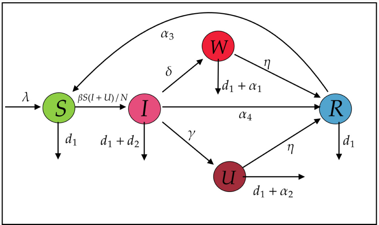
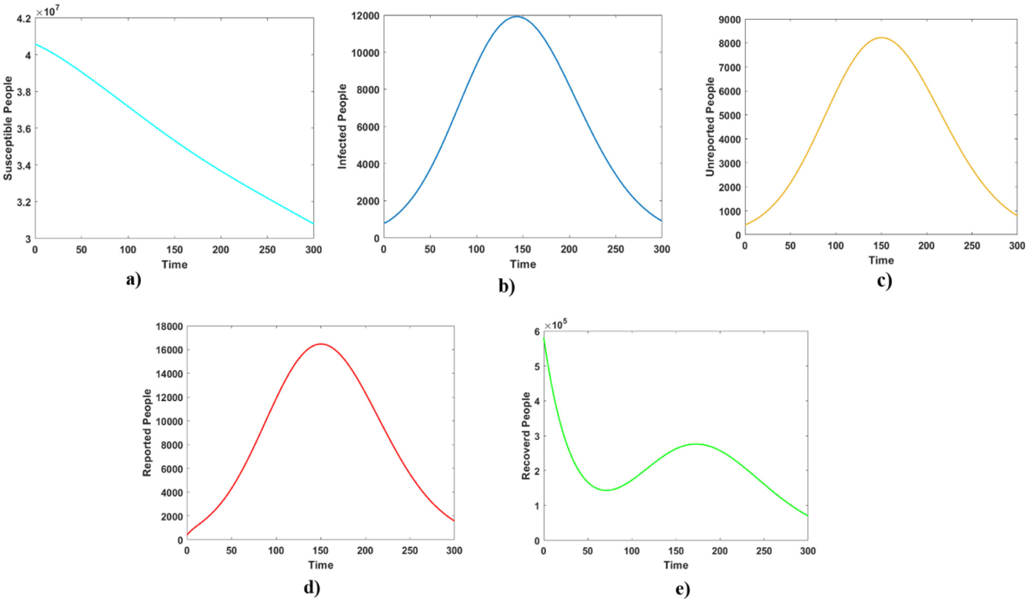
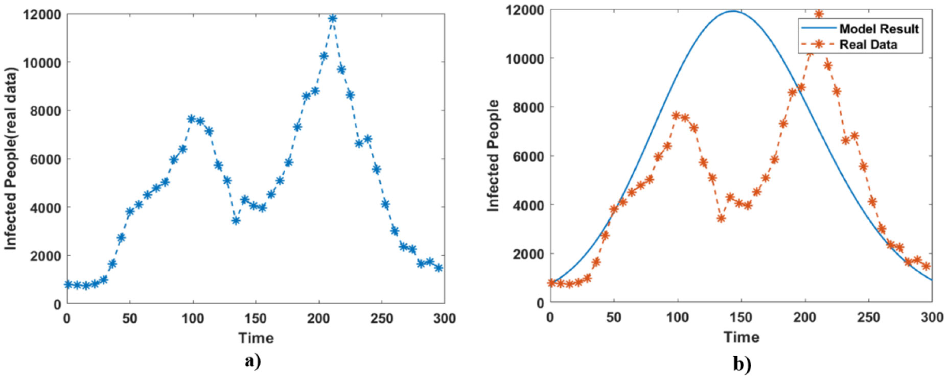
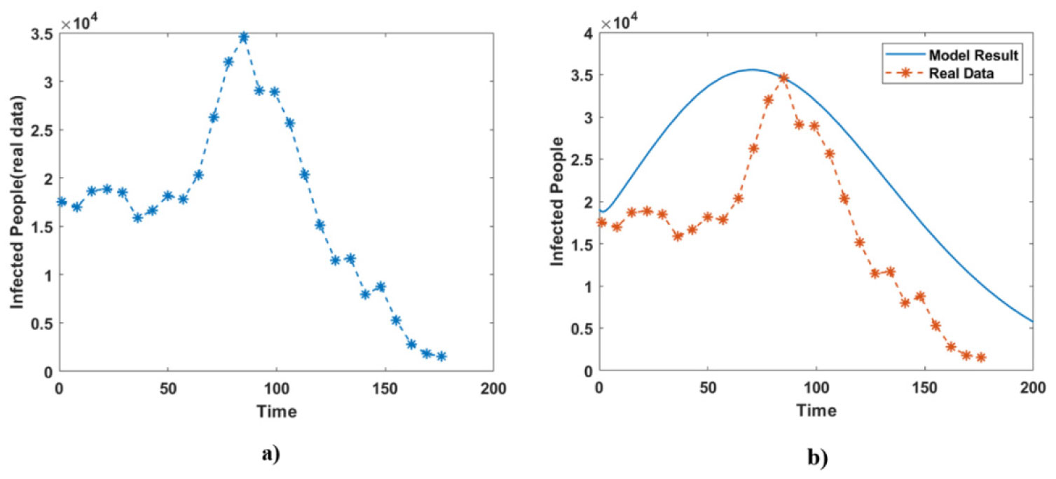
Spreading COVID-19 pandemic has been considered as a global issue. Many international efforts including mathematical approaches have been recently discussed to control this disease more effectively. In this study, we have developed our previous SIUWR model and some transmission parameters are added. Accordingly, the basic reproduction number and elasticity coefficients are calculated at the equilibrium points. Then, some key critical model parameters are identified based on local sensitivities. In addition, the validation of the suggested model is checked by comparing some collected real data in Iraq and France from January 1st, 2021 to December 25th, 2021. Interestingly, there are good agreements between the model results and the real confirmed data using computational simulations in MATLAB. Results provide some biological interpretations and they can be used to control this pandemic more effectively. The model results will be used for both countries in minimizing the impact of this virus on their communities.

| [1] | Ali DS, Othman HO (2021) Pharmacological insight into possible treatment agents for the lethal covid-19 pandemic in Kurdistan Region-Iraq. Sys Rev Pharm 12: 786-804. |
| [2] | Prague M, Wittkop L, Collin A, et al. (2020) Population modeling of early COVID-19 epidemic dynamics in French regions and estimation of the lockdown impact on infection rate. medRxiv: 2020.04.21.20073536 . https://doi.org/10.1101/2020.04.21.20073536 |
| [3] |
Ivorra B, Ferrández MR, Vela-Pérez M, et al. (2020) Mathematical modeling of the spread of the coronavirus disease 2019 (COVID-19) taking into account the undetected infections. The case of China. Commun Nonlinear Sci 88: 105303. https://doi.org/10.1016/j.cnsns.2020.105303 
|
| [4] | Aries N, Ounis H Mathematical modeling of COVID-19 pandemic in the African continent (2020). https://doi.org/10.1101/2020.10.10.20210427 |
| [5] |
Bugalia S, Bajiya VP, Tripathi JP, et al. (2020) Mathematical modeling of COVID-19 transmission: the roles of intervention strategies and lockdown. Math Biosci Eng 17: 5961-5986. https://doi.org/10.3934/mbe.2020318
|
| [6] |
Khoshnaw SHA, Shahzad M, Ali M, et al. (2020) A quantitative and qualitative analysis of the COVID–19 pandemic model. Chaos Soliton Fract 138: 109932. https://doi.org/10.1016/j.chaos.2020.109932
|
| [7] | Mamo DK, Koya PR (2015) Mathematical modeling and simulation study of SEIR disease and data fitting of Ebola epidemic spreading in West Africa. JMEST 2: 106-114. |
| [8] |
Ibrahim MA, Al-Najafi A (2020) Modeling, control, and prediction of the spread of COVID-19 using compartmental, logistic, and gauss models: a case study in Iraq and Egypt. Processes 8: 1400. https://doi.org/10.3390/pr8111400
|
| [9] |
Alqarni MS, Alghamdi M, Muhammad T, et al. (2022) Mathematical modeling for novel coronavirus (COVID-19) and control. Numer Meth Part D E 38: 760-776. https://doi.org/10.1002/num.22695
|
| [10] |
Farman M, Akgül A, Nisar KS, et al. (2022) Epidemiological analysis of fractional order COVID-19 model with Mittag-Leffler kernel. AIMS Mathematics 7: 756-783. https://doi.org/10.3934/math.2022046
|
| [11] |
Danane J, Allali K, Hammouch Z, et al. (2021) Mathematical analysis and simulation of a stochastic COVID-19 Lévy jump model with isolation strategy. Results Phys 23: 103994. https://doi.org/10.1016/j.rinp.2021.103994
|
| [12] |
Hussain G, Khan T, Khan A, et al. (2021) Modeling the dynamics of novel coronavirus (COVID-19) via stochastic epidemic model. Alex Eng J 60: 4121-4130. https://doi.org/10.1016/j.aej.2021.02.036
|
| [13] |
Singh H, Srivastava HM, Hammouch Z, et al. (2021) Numerical simulation and stability analysis for the fractional-order dynamics of COVID-19. Results Phys 20: 103722. https://doi.org/10.1016/j.rinp.2020.103722
|
| [14] |
Baba IA, Yusuf A, Nisar KS, et al. (2021) Mathematical model to assess the imposition of lockdown during COVID-19 pandemic. Results Phys 20: 103716. https://doi.org/10.1016/j.rinp.2020.103716
|
| [15] |
Noor MA, Raza A, Arif MS, et al. (2022) Non-standard computational analysis of the stochastic Covid-19 pandemic model: an application of computational biology. Alex Eng J 61: 619-630. https://doi.org/10.1016/j.aej.2021.06.039
|
| [16] |
Khajanchi S, Sarkar K, Mondal J, et al. (2021) Mathematical modeling of the COVID-19 pandemic with intervention strategies. Results Phys 25: 104285. https://doi.org/10.1016/j.rinp.2021.104285
|
| [17] |
Baba IA, Ahmed I, Al-Mdallal QM, et al. (2022) Numerical and theoretical analysis of an awareness COVID-19 epidemic model via generalized Atangana-Baleanu fractional derivative. J Appl Math Comp Mec 21: 7-18. https://doi.org/10.17512/jamcm.2022.1.01
|
| [18] | Baba IA, Sani MA, Nasidi BA (2021) Fractional dynamical model to assess the efficacy of facemask to the community transmission of COVID-19. Comput Method Biomec 2021: 1-11. https://doi.org/10.1080/10255842.2021.2024170 |
| [19] |
Musa SS, Baba IA, Yusuf A, et al. (2021) Transmission dynamics of SARS-CoV-2: A modeling analysis with high-and-moderate risk populations. Results Phys 26: 104290. https://doi.org/10.1016/j.rinp.2021.104290
|
| [20] | Baba I A, Baleanu D Awareness as the most effective measure to mitigate the spread of COVID-19 in Nigeria (2020). http://hdl.handle.net/20.500.12416/4548 |
| [21] |
Kouidere A, Youssoufi LEL, Ferjouchia H, et al. (2021) Optimal control of mathematical modeling of the spread of the COVID-19 pandemic with highlighting the negative impact of quarantine on diabetics people with Cost-effectiveness. Chaos Soliton Fract 145: 110777. https://doi.org/10.1016/j.chaos.2021.110777
|
| [22] |
Kouidere A, Kada D, Balatif O, et al. (2021) Optimal control approach of a mathematical modeling with multiple delays of the negative impact of delays in applying preventive precautions against the spread of the COVID-19 pandemic with a case study of Brazil and cost-effectiveness. Chaos Soliton Fract 142: 110438. https://doi.org/10.1016/j.chaos.2020.110438
|
| [23] |
Aldila D, Shahzad M, Khoshnaw SHA, et al. (2022) Optimal control problem arising from COVID-19 transmission model with rapid-test. Results Phys 2022: 105501. https://doi.org/10.1016/j.rinp.2022.105501
|
| [24] | Rasool HM, Khoshnaw SHA (2021) Techniques of model reductions in biochemical cell signaling pathways. arXiv: 2109.06566 . https://doi.org/10.48550/arXiv.2109.06566 |
| [25] |
Akgül A, Khoshnaw SHA, Abdalrahman AS (2020) Mathematical modeling for enzyme inhibitors with slow and fast subsystems. Arab J Basic Appl Sci 27: 442-449. https://doi.org/10.1080/25765299.2020.1844369
|
| [26] | Khoshnaw SHA, Rasool HM (2019) Mathematical modelling for complex biochemical networks and identification of fast and slow reactions. Mathematical Methods and Modelling in Applied Sciences . Cham: Springer 55-69. https://doi.org/10.1007/978-3-030-43002-3_6 |
| [27] | Khoshnaw SHA (2015) Model reductions in biochemical reaction networks[PhD thesis]. United Kingdom: University of Leicester. |
| [28] | WHO-COVID-19-global-data, 2020. Available from: https://covid19.who.int/WHO-COVID-19-global-data.csv |
| [29] |
Diekmann O, Heesterbeek JAP, Roberts MG (2010) The construction of next-generation matrices for compartmental epidemic models. J R Soc Interface 7: 873-885. https://doi.org/10.1098/rsif.2009.0386
|
| [30] |
Perasso A (2018) An introduction to the basic reproduction number in mathematical epidemiology. ESAIM: ProcS 62: 123-138. https://doi.org/10.1051/proc/201862123
|
| [31] |
Hartemink NA, Randolph SE, Davis SA, et al. (2008) The basic reproduction number for complex disease systems: Defining R0 for tick-borne infections. Am Nat 171: 743-754. https://doi.org/10.1086/587530
|
| [32] |
Van den Driessche P, Watmough J (2008) Further notes on the basic reproduction number. Mathematical Epidemiology . Heidelberg: Springer Berlin 159-178. https://doi.org/10.1007/978-3-540-78911-6_6
|
| [33] |
Yang HM (2014) The basic reproduction number obtained from Jacobian and next generation matrices–A case study of dengue transmission modelling. Biosystems 126: 52-75. https://doi.org/10.1016/j.biosystems.2014.10.002
|
| [34] |
Fosu GO, Akweittey E, Adu-Sackey A (2020) Next-generation matrices and basic reproductive numbers for all phases of the Coronavirus disease. Open J Math Sci 4: 261-272. https://doi.org/10.30538/oms2020.0117
|
| [35] |
Rahman B, Khoshnaw SHA, Agaba GO, et al. (2021) How containment can effectively suppress the outbreak of COVID-19: a mathematical modeling. Axioms 10: 204. https://doi.org/10.3390/axioms10030204
|
| [36] |
Aldila D, Samiadji BM, Simorangkir GM, et al. (2021) Impact of early detection and vaccination strategy in COVID-19 eradication program in Jakarta, Indonesia. BMC Res Notes 14: 1-7. https://doi.org/10.1186/s13104-021-05540-9
|
| [37] |
Alimohamadi Y, Taghdir M, Sepandi M (2020) Estimate of the basic reproduction number for COVID-19: a systematic review and meta-analysis. J Prev Med Public Health 53: 151-157. https://doi.org/10.3961/jpmph.20.076
|
| [38] |
Aldila D, Khoshnaw SHA, Safitri E, et al. (2020) A mathematical study on the spread of COVID-19 considering social distancing and rapid assessment: The case of Jakarta, Indonesia. Chaos Soliton Fract 139: 110042. https://doi.org/10.1016/j.chaos.2020.110042
|
 bioeng-09-02-014-s001.pdf bioeng-09-02-014-s001.pdf |
 |

Figures(6) / Tables(2)

Bashdar A. Salam, Sarbaz H. A. Khoshnaw, Abubakr M. Adarbar, Hedayat M. Sharifi, Azhi S. Mohammed. Model predictions and data fitting can effectively work in spreading COVID-19 pandemic[J]. AIMS Bioengineering, 2022, 9(2): 197-212. doi: 10.3934/bioeng.2022014


 DownLoad: