A literature review on COVID-19 disease diagnosis from respiratory sound data

Kranthi Kumar Lella; Alphonse PJA; Kranthi Kumar Lella; Alphonse PJA

doi:10.3934/bioeng.2021013

AIMS Bioengineering

2021, Volume 8, Issue 2: 140-153. doi: 10.3934/bioeng.2021013

Previous Article Next Article

Mini review Special Issues

A literature review on COVID-19 disease diagnosis from respiratory sound data

Kranthi Kumar Lella ,
Alphonse PJA ^,

Department of Computer Applications, NIT Tiruchirappalli, Tamil Nadu, India-620015

Received: 12 January 2021 Accepted: 25 February 2021 Published: 05 March 2021

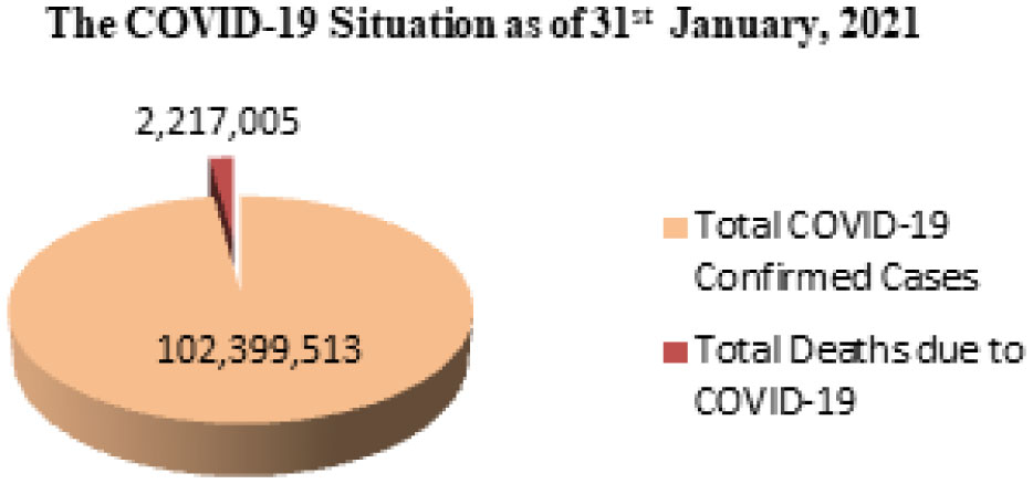
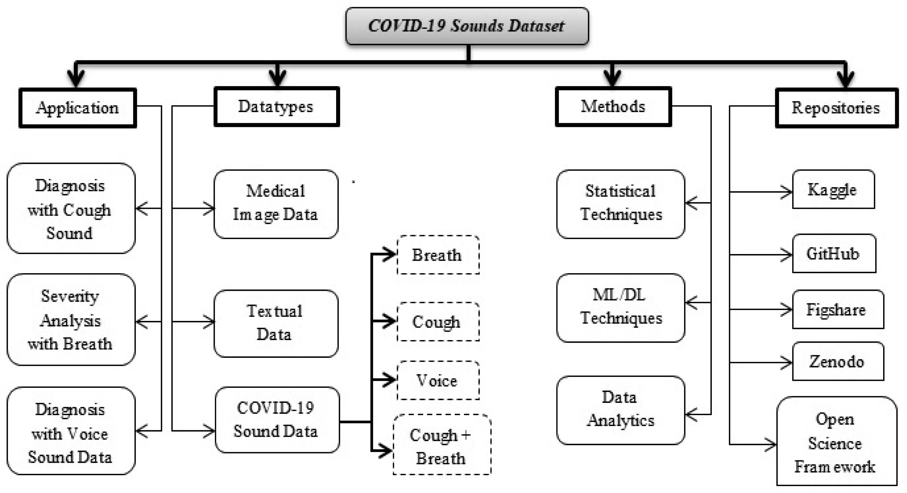
The World Health Organization (WHO) has announced a COVID-19 was a global pandemic in March 2020. It was initially started in china in the year 2019 December and affected an expanding number of nations in various countries in the last few months. In this particular situation, many techniques, methods, and AI-based classification algorithms are put in the spotlight in reacting to fight against it and reduce the rate of such a global health crisis. COVID-19's main signs are heavy temperature, different cough, cold, breathing shortness, and a combination of loss of sense of smell and chest tightness. The digital world is growing day by day; in this context digital stethoscope can read all of these symptoms and diagnose respiratory disease. In this study, we majorly focus on literature reviews of how SARS-CoV-2 is spreading and in-depth analysis of the diagnosis of COVID-19 disease from human respiratory sounds like cough, voice, and breath by analyzing the respiratory sound parameters. We hope this review will provide an initiative for the clinical scientists and researcher's community to initiate open access, scalable, and accessible work in the collective battle against COVID-19.
- COVID-19,
- World Health Organization,
- machine learning,
- deep learning,
- artificial intelligence,
- respiratory sounds
Citation: Kranthi Kumar Lella, Alphonse PJA. A literature review on COVID-19 disease diagnosis from respiratory sound data[J]. AIMS Bioengineering, 2021, 8(2): 140-153. doi: 10.3934/bioeng.2021013

Related Papers:

Abstract

The World Health Organization (WHO) has announced a COVID-19 was a global pandemic in March 2020. It was initially started in china in the year 2019 December and affected an expanding number of nations in various countries in the last few months. In this particular situation, many techniques, methods, and AI-based classification algorithms are put in the spotlight in reacting to fight against it and reduce the rate of such a global health crisis. COVID-19's main signs are heavy temperature, different cough, cold, breathing shortness, and a combination of loss of sense of smell and chest tightness. The digital world is growing day by day; in this context digital stethoscope can read all of these symptoms and diagnose respiratory disease. In this study, we majorly focus on literature reviews of how SARS-CoV-2 is spreading and in-depth analysis of the diagnosis of COVID-19 disease from human respiratory sounds like cough, voice, and breath by analyzing the respiratory sound parameters. We hope this review will provide an initiative for the clinical scientists and researcher's community to initiate open access, scalable, and accessible work in the collective battle against COVID-19.

Conflict of interest

The authors declared no conflict of interest.

Author contributions

Kranthi Kumar Lella: Original draft preparation, Formal Analysis, and Data Conceptualization. Alphonse PJA: Supervision, Reviewing, and Editing.

References

[1]	World Health Organization Coronavirus disease 2019 (covid-19) (2020) .Available from: https://www.who.int/.
[2]	Wang Y, Hu M, Li Q, et al. (2020) Abnormal respiratory patterns classifier may contribute to large-scale screening of people infected with COVID-19 in an accurate and unobtrusive manner. arXiv: 2002.05534 .
[3]	Jiang Z, Hu M, Fan L, et al. (2020) Combining visible light and infrared imaging for efficient detection of respiratory infections such as COVID-19 on portable device. arXiv: 2004.06912 .
[4]	Shuja J, Alanazi E, Alasmary W, et al. Covid-19 open source data sets: a comprehensive survey (2020) . doi: 10.1101/2020.05.19.20107532
[5]	Rasheed J, Jamil A, Hameed AA, et al. (2020) A survey on artificial intelligence approaches in supporting frontline workers and decision makers for COVID-19 pandemic. Chaos Soliton Fract 2020: 110337. doi: 10.1016/j.chaos.2020.110337
[6]	Alafif T, Tehame AM, Bajaba S, et al. Machine and deep learning towards COVID-19 diagnosis and treatment: survey, challenges, and future directions (2020) . doi: 10.13140/RG.2.2.20805.47848/1
[7]	Gramming P, Sundberg J, Ternström S, et al. (1988) Relationship between changes in voice pitch and loudness. J Voice 2: 118-126. doi: 10.1016/S0892-1997(88)80067-5
[8]	Imran A, Posokhova I, Qureshi HN, et al. AI4COVID-19: AI-enabled preliminary diagnosis for COVID-19 from cough samples via an app (2020) . doi: 10.1016/j.imu.2020.100378
[9]	Brown C, Chauhan J, Grammenos A, et al. Exploring automatic diagnosis of covid-19 from crowdsourced respiratory sound data (2020) . doi: 10.1145/3394486.3412865
[10]	Hassan A, Shahin I, Alsabek MB Covid-19 detection system using recurrent neural networks (2020) . doi: 10.1109/CCCI49893.2020.9256562
[11]	Zhao W, Singh R Speech-based parameter estimation of an asymmetric vocal fold oscillation model and its application in discriminating vocal fold pathologies (2020) . doi: 10.1109/ICASSP40776.2020.9052984
[12]	Singh R (2019) Production and perception of voice. Profiling Humans from their Voice Singapore: Springer, 27-83. doi: 10.1007/978-981-13-8403-5_2
[13]	Shereen MA, Khan S, Kazmi A, et al. (2020) COVID-19 infection: Origin, transmission, and characteristics of human coronaviruses. J Adv Res 24: 91-98. doi: 10.1016/j.jare.2020.03.005
[14]	Ilyas S, Srivastava RR, Kim H (2020) Disinfection technology and strategies for COVID-19 hospital and bio-medical waste management. Sci Total Environ 749: 141652. doi: 10.1016/j.scitotenv.2020.141652
[15]	Shobhana R, Bharat LS Novel coronavirus disease 2019 (COVID-19) pandemic: Considerations for the biomedical waste sector in India (2020) . doi: 10.1016/j.cscee.2020.100029
[16]	Das A, Garg R, Ojha B, et al. (2020) Biomedical waste management: The challenge amidst COVID-19 pandemic. J Lab Physicians 12: 161-162. doi: 10.1055/s-0040-1716662
[17]	Filimonau V The prospects of waste management in the hospitality sector post-COVID-19 (2020) . doi: 10.1016/j.resconrec.2020.105272
[18]	Kulkarni BN, Anantharama V (2020) Repercussions of COVID-19 pandemic on municipal solid waste management: challenges and opportunities. Sci Total Environ 743: 140693. doi: 10.1016/j.scitotenv.2020.140693
[19]	Sharma HB, Vanapalli KR, Cheela VRS, et al. (2020) Challenges, opportunities, and innovations for effective solid waste management during and post COVID-19 pandemic. Resour Conserv Recy 162: 105052. doi: 10.1016/j.resconrec.2020.105052
[20]	Ganguly RK, Chakraborty SK Integrated approach in municipal solid waste management in COVID-19 pandemic: Perspectives of a developing country like India in a global scenario (2021) . doi: 10.1016/j.cscee.2021.100087
[21]	Adam JP, Khazaka M, Charikhi F, et al. Management of human resources of a pharmacy department during the COVID-19 pandemic: take a ways from the first wave (2021) . doi: 10.1016/j.sapharm.2020.10.014
[22]	Orlandic L, Teijeiro T, Atienza D (2020) The COUGHVID crowdsourcing dataset: A corpus for the study of large-scale coughs analysis algorithms. arXiv: 2009.11644 . doi: 10.5281/zenodo.4048312
[23]	Bader M, Shahin I, Hassan A (2020) Studying the similarity of COVID-19 sounds based on correlation analysis of MFCC. arXiv: 2010.08770 . doi: 10.1109/CCCI49893.2020.9256700
[24]	Ismail MA, Deshmukh S, Singh R (2020) Detection of COVID-19 through the analysis of vocal fold oscillations. arXiv: 2010.10707 .
[25]	Chaudhari G, Jiang X, Fakhry A, et al. (2020) Virufy: Global applicability of crowdsourced and clinical datasets for AI detection of COVID-19 from cough. arXiv: 2011.13320 .
[26]	Laguarta J, Hueto F, Subirana B COVID-19 artificial intelligence diagnosis using only cough recordings (2020) . doi: 10.1109/OJEMB.2020.3026928
[27]	Quartieri TF, Talker T, Palmer JS A framework for biomarkers of COVID-19 based on coordination of speech-production subsystems (2020) . doi: 10.1109/OJEMB.2020.2998051
[28]	Han J, Qian K, Song M, et al. (2020) An early study on intelligent analysis of speech under covid-19: Severity, sleep quality, fatigue, and anxiety. arXiv: 2005.00096 . doi: 10.21437/Interspeech.2020-2223
[29]	Ritwik KVS, Kalluri SB, Vijayasenan D (2020) COVID-19 patient detection from telephone quality speech data. arXiv: 2011.04299 .

Reader Comments

Your name:*

Email:*
© 2021 the Author(s), licensee AIMS Press. This is an open access article distributed under the terms of the Creative Commons Attribution License (http://creativecommons.org/licenses/by/4.0)