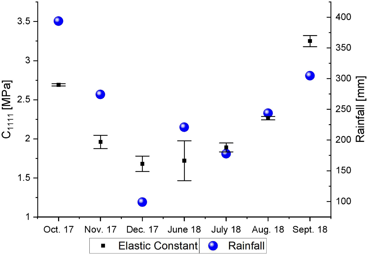
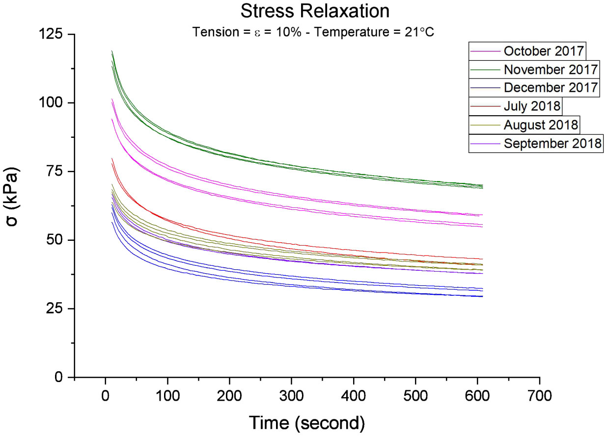
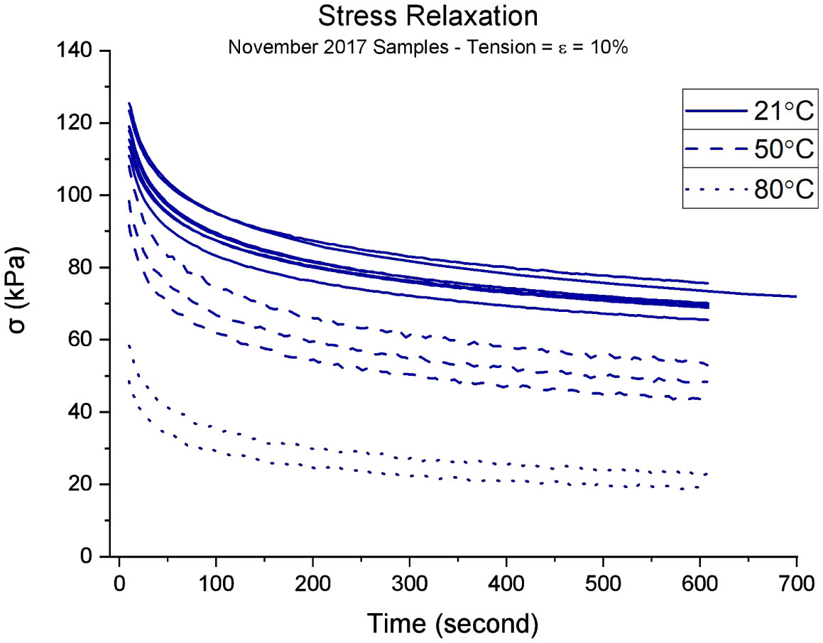
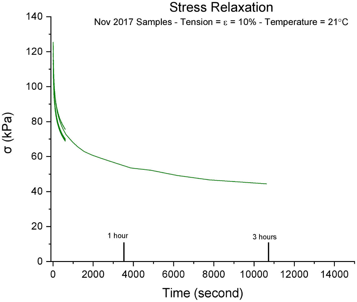
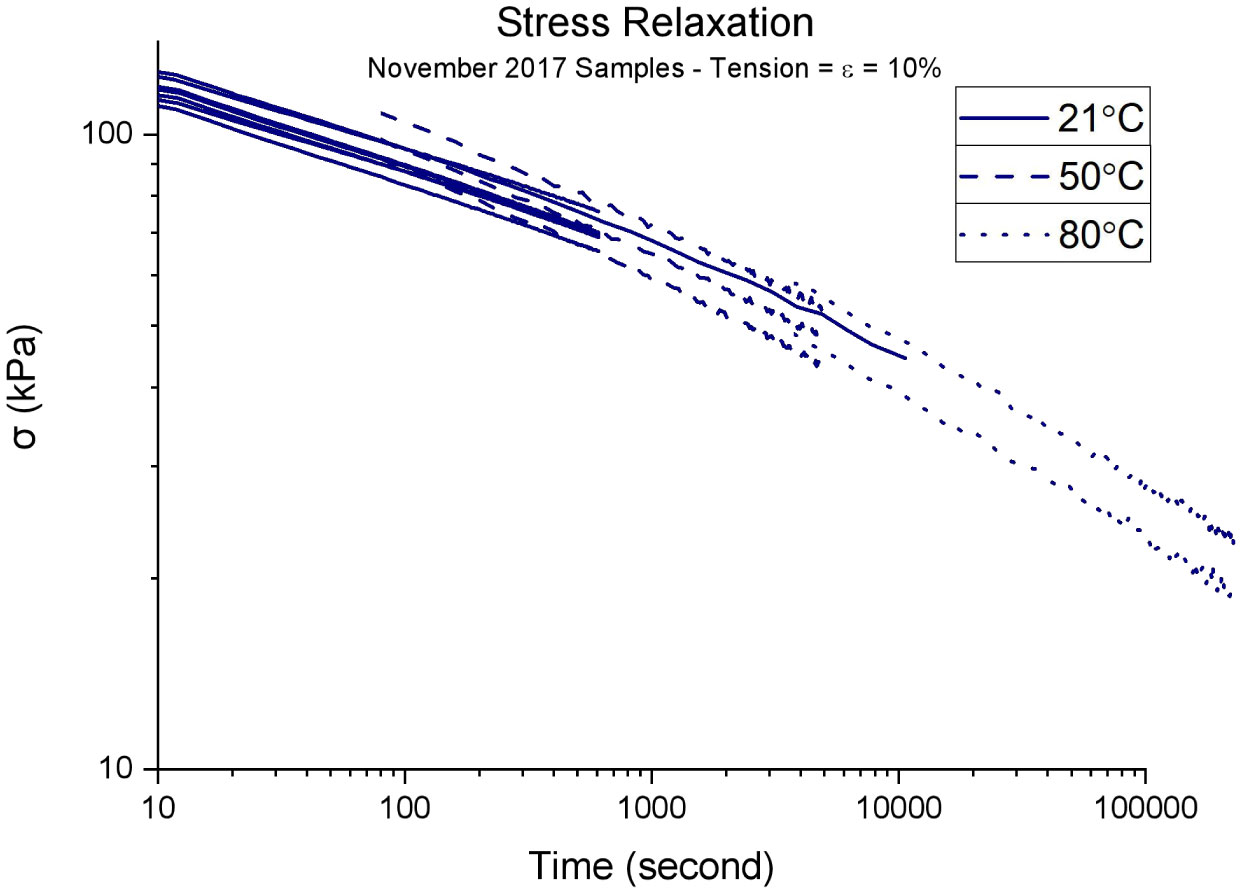
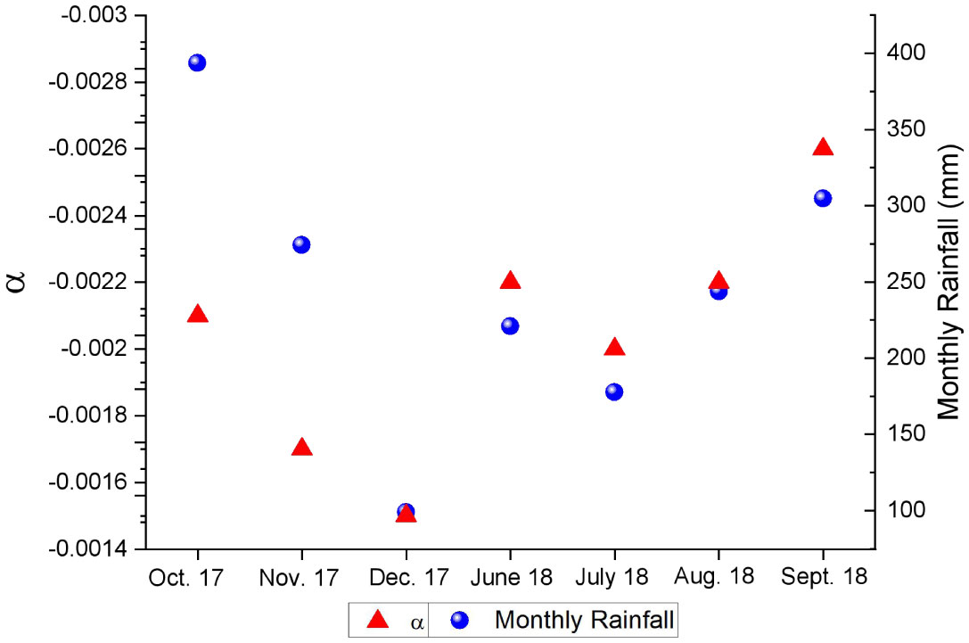
The Sociedad de Caucho Colombo Argentina (SOCCA) collected natural rubber (NR) from Yarima, Colombia, for seven months spanning two years. The unvulcanized NR was used to conduct a preliminary study, part of a long-term study, to uncover some underlying mechanisms in charge of imparting variation between NR batches, such as the collection site's rainfall conditions and storage period by using calorimetry, rheometry, and a dynamic mechanical analyzer. The ultrasound study found that an increase in monthly rainfall increased the material's elastic constant at 10 MHz, and the crystallization study uncovered that the amount of crystallization decreased with increased rain while remaining relatively constant if rainfall was within the recommended rainfall amount for the tree. Additionally, stress relaxation measurements revealed that an increase in rainfall suggested an increase in the material's temperature sensitivity. The temperature sensitivity relates to the material's processability in which an increase in temperature with high sensitivity will have a more drastic decrease in stress during a relaxation test compared to a material with low sensitivity.
Citation: Allen Jonathan Román, Jamelah Zena Travis, Juan Carlos Martínez Ávila, Tim A. Osswald. Influence of plantation climate and storage time on thermal and viscoelastic properties of natural rubber[J]. AIMS Bioengineering, 2021, 8(1): 95-111. doi: 10.3934/bioeng.2021010
The Sociedad de Caucho Colombo Argentina (SOCCA) collected natural rubber (NR) from Yarima, Colombia, for seven months spanning two years. The unvulcanized NR was used to conduct a preliminary study, part of a long-term study, to uncover some underlying mechanisms in charge of imparting variation between NR batches, such as the collection site's rainfall conditions and storage period by using calorimetry, rheometry, and a dynamic mechanical analyzer. The ultrasound study found that an increase in monthly rainfall increased the material's elastic constant at 10 MHz, and the crystallization study uncovered that the amount of crystallization decreased with increased rain while remaining relatively constant if rainfall was within the recommended rainfall amount for the tree. Additionally, stress relaxation measurements revealed that an increase in rainfall suggested an increase in the material's temperature sensitivity. The temperature sensitivity relates to the material's processability in which an increase in temperature with high sensitivity will have a more drastic decrease in stress during a relaxation test compared to a material with low sensitivity.
Natural Rubber
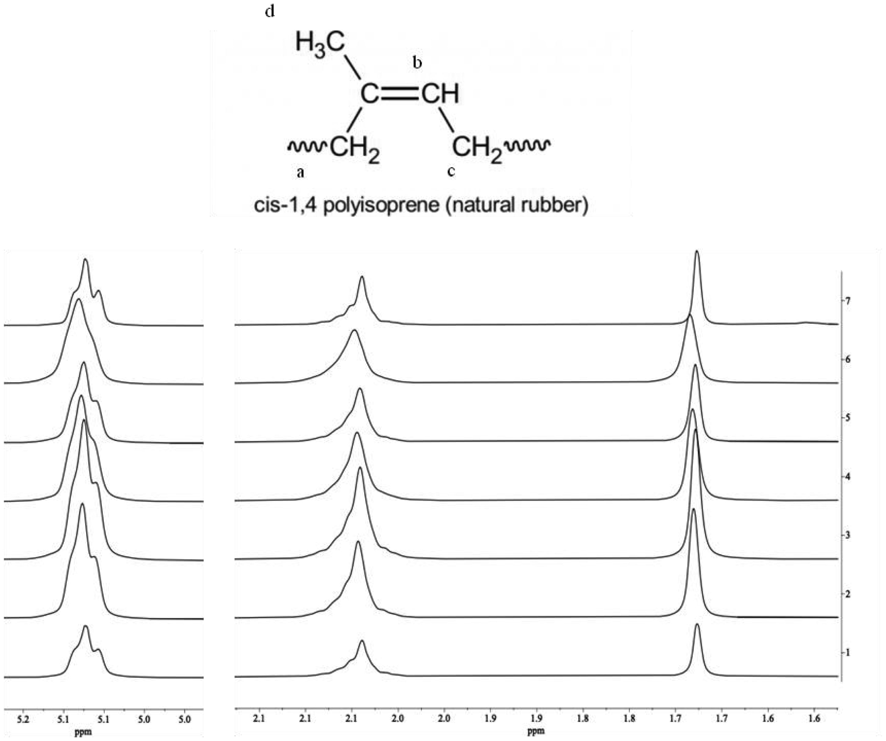
Proton Nuclear Magnetic Resonance
Dynamic Mechanical Analyzer
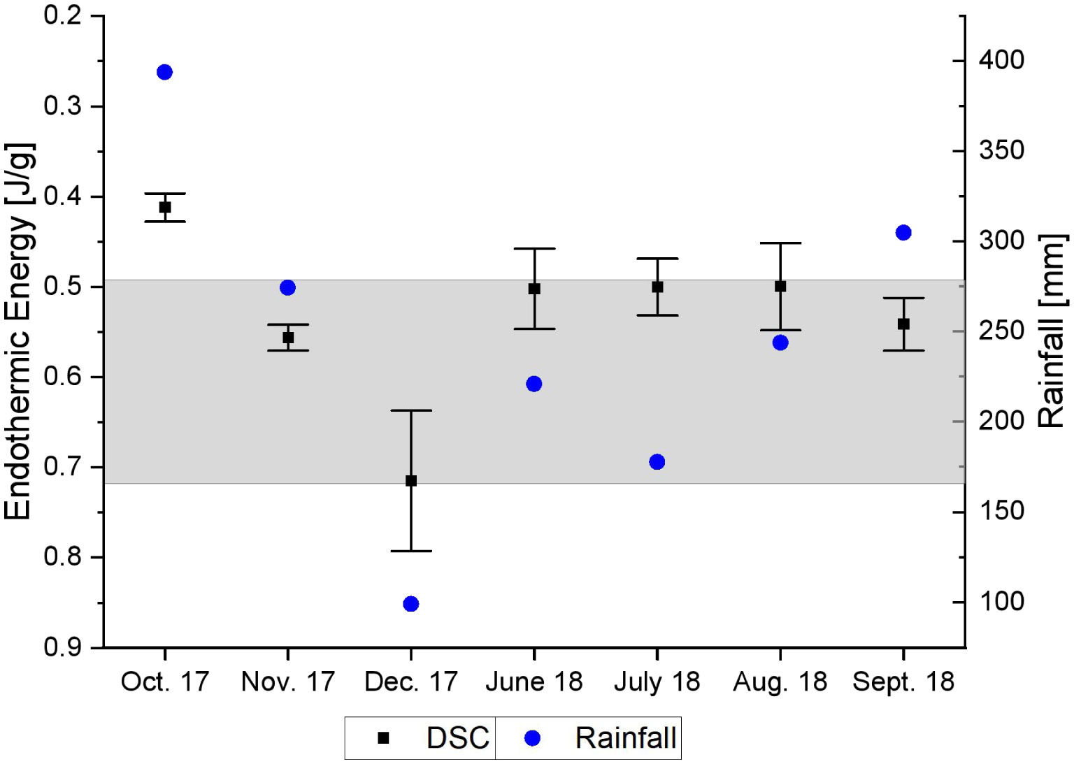
Differential Scanning Calorimetry
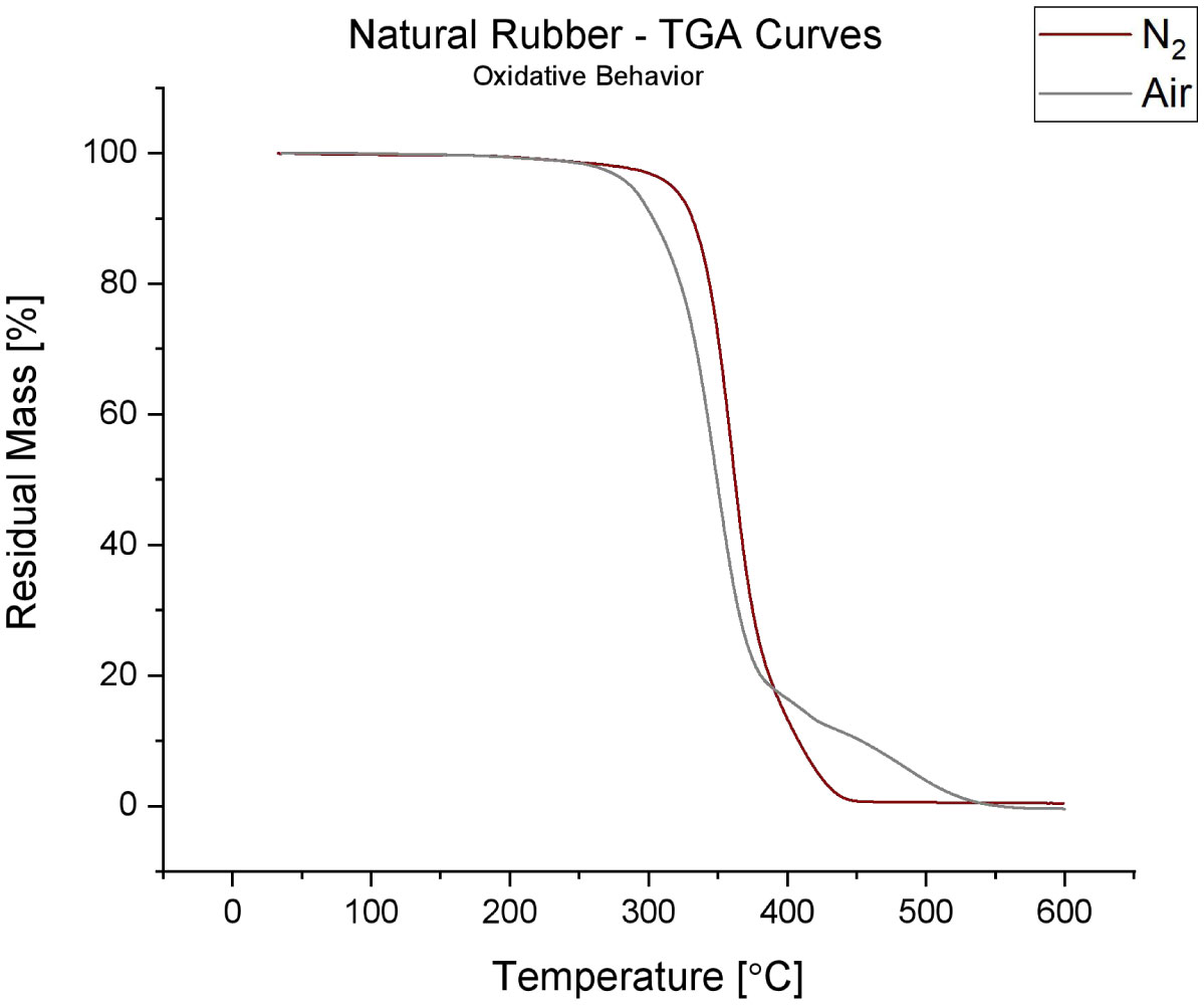
Thermogravimetric analysis

| [1] |
Umar HY, Okore NE, Toryila M, et al. Evaluation of impact of climatic factors on latex yield of hevea brasiliensis (2017) . doi: 10.20431/2454-6224.0305004

|
| [2] | Rao P, Vijayakumar KR (1992) Natural rubber: Biology, Cultivation and Technology Development in Crop Science Elsevier Science. |
| [3] |
Mesike CS, Esekhade TU (2014) Rainfall variability and rubber production in Nigeria. Afr J Environ Sci Technol 8: 54-57. doi: 10.5897/AJEST2013.1593
|
| [4] |
Kenneth OO, Okeoghene AE (2006) Evaluation of five weather characters on latex yield in hevea brasiliensis. Int J Agr Res 1: 234-239. doi: 10.3923/ijar.2006.234.239
|
| [5] |
Craciun G, Manaila E, Stelescu MD (2016) New elastomeric materials based on natural rubber obtained by electron beam irradiation for food and pharmaceutical use. Materials 9: 999. doi: 10.3390/ma9120999
|
| [6] |
Osswald TA (2017) Understanding Polymer Processing München: Carl Hanser Verlag GmbH Publications. doi: 10.3139/9781569906484
|
| [7] |
Kuang X, Chen K, Dunn CK, et al. (2018) 3D printing of highly stretchable, shape-memory, and self-healing elastomer toward novel 4D printing. ACS Appl Mater Interfaces 10: 7381-7388. doi: 10.1021/acsami.7b18265
|
| [8] |
Choi JH, Kang HJ, Jeong HY, et al. (2005) Heat aging effects on material property and the fatigue life of vulcanized natural rubber, and fatigue life prediction equations. J Mech Sci Technol 19: 1229-1242. doi: 10.1007/BF02984044
|
| [9] |
Martinez JRS, Le Cam JB, Balandraud X, et al. (2013) Mechanisms of deformation in crystallizable natural rubber. Part 1: thermal characterization. Polymer 54: 2717-2726. doi: 10.1016/j.polymer.2013.03.011
|
| [10] |
Brüning K, Schneider K, Roth SV, et al. (2012) Kinetics of strain-induced crystallization in natural rubber studied by WAXD: dynamic and impact tensile experiments. Macromolecules 45: 7914-7919. doi: 10.1021/ma3011476
|
| [11] | Wei Y, Zhang H, Wu L, et al. (2017) A review on characterization of molecular structure of natural rubber. MOJ Poly Sci 1: 197-199. |
| [12] |
Kitaura T, Kobayashi M, Tarachiwin L, et al. (2018) Characterization of natural rubber end groups using high-sensitivity NMR. Macromol Chem Phys 219: 1700331. doi: 10.1002/macp.201700331
|
| [13] | Sakdapipanich JT, Rojruthai P (2012) Molecular structure of natural rubber and its characteristics based on recent evidence. Biotechnology-Molecular Studies and Novel Applications for Improved Quality of Human Life Croatia: InTech, 213. |
| [14] |
Tanaka Y (2001) Structural characterization of natural polyisoprenes: Solve the mystery of natural rubber based on structural study. Rubber Chem Technol 74: 355-375. doi: 10.5254/1.3547643
|
| [15] |
Tanaka Y, Sato H, Kageyu A (1983) Structure and biosynthesis mechanism of natural cis-polyisoprene from Goldenrod. Rubber Chem Technol 56: 299-303. doi: 10.5254/1.3538125
|
| [16] |
Tangpakdee J, Tanaka Y, Ogura K, et al. (1997) Structure of in vitro synthesized rubber from fresh bottom fraction of Hevea latex. Phytochemistry 45: 275-281. doi: 10.1016/S0031-9422(96)00839-4
|
| [17] | James CR (1984) NMR and Macromolecules Washington: American Chemical Society. |
| [18] |
Tanaka Y, Takeuchi Y, Kobayashi M, et al. (1971) Characterization of diene polymers. I. Infrared and NMR studies: nonadditive behavior of characteristic infrared bands. J Polym Sci Pol Phys 9: 43-57. doi: 10.1002/pol.1971.160090104
|
| [19] |
Sato H, Tanaka Y (1979) 1H-NMR study of polyisoprenes. Polym Sci: Polym Chem Ed 17: 3551-3558. doi: 10.1002/pol.1979.170171113
|
| [20] |
Sotta P, Albouy PA (2020) Strain-induced crystallization in natural rubber: flory's theory revisited. Macromolecules 53: 3097-3109. doi: 10.1021/acs.macromol.0c00515
|
| [21] |
Lakes RS (2004) Viscoelastic measurement techniques. Rev Sci Instrum 75: 797-810. doi: 10.1063/1.1651639
|
| [22] | Bruker (2014) Bruker Avance Beginners Guide Bruker Corporation Publishing, 23-30. |
| [23] |
Chen HY (1962) Determination of cis-1,4 and trans-1,4 contents of polyisoprenes by high resolution nuclear magnetic resonance. Anal Chem 34: 1793-1795. doi: 10.1021/ac60193a038
|
| [24] |
Basfar AA, Abdel-Aziz MM, Mofti S (2002) Influence of different curing systems on the physico-mechanical properties and stability of SBR and NR rubbers. Radiat Phys Chem 63: 81-87. doi: 10.1016/S0969-806X(01)00486-8
|
| [25] |
Gooding EGB (1952) Studies in the Physiology of Latex III. Effects of Various Factors on the Concentration of Latex of Hevea brasiliensis. New Phytol 51: 139-153. doi: 10.1111/j.1469-8137.1952.tb06122.x
|
| [26] |
Ellis EC, Turgeon R, Spanswick RM (1992) Quantitative analysis of photosynthate unloading in developing seeds of phaseolus vulgaris L.: II. pathway and turgor sensitivity. Plant Physiol 99: 643-651. doi: 10.1104/pp.99.2.643
|
| [27] |
Niklas KJ (1989) Mechanical behavior of plant tissues as inferred from the theory of pressurized cellular solids. Am J Bot 76: 929-937. doi: 10.1002/j.1537-2197.1989.tb15071.x
|
| [28] | Osswald TA, Rudolph N (2015) Polymer Rheology München: Carl Hanser Verlag GmbH Publications. |
| [29] |
Minoura Y, Kamagata K (1964) Stress relaxation of raw natural rubber. J Appl Polym Sci 8: 1077-1087. doi: 10.1002/app.1964.070080305
|
| [30] |
Tosaka M, Kawakami D, Senoo K, et al. (2006) Crystallization and stress relaxation in highly stretched samples of natural rubber and its synthetic analogue. Macromolecules 39: 5100-5105. doi: 10.1021/ma060407+
|
| [31] |
Lakes R, Lakes RS (2009) Viscoelastic Materials UK: Cambridge University Press. doi: 10.1017/CBO9780511626722
|
| [32] |
Tzoganakis C, Vlachopoulos J, Hamielec AE (1988) Production of controlled-rheology polypropylene resins by peroxide promoted degradation during extrusion. Polym Eng Sci 28: 170-180. doi: 10.1002/pen.760280308
|
| [33] | Wainwright-Déri E Rubber–does ‘natural’ mean sustainable? (2018) .Available from: https://www.spott.org/news/rubber-does-natural-mean-sustainable/. |
Figures(13) / Tables(2)

Allen Jonathan Román, Jamelah Zena Travis, Juan Carlos Martínez Ávila, Tim A. Osswald. Influence of plantation climate and storage time on thermal and viscoelastic properties of natural rubber[J]. AIMS Bioengineering, 2021, 8(1): 95-111. doi: 10.3934/bioeng.2021010


 DownLoad: