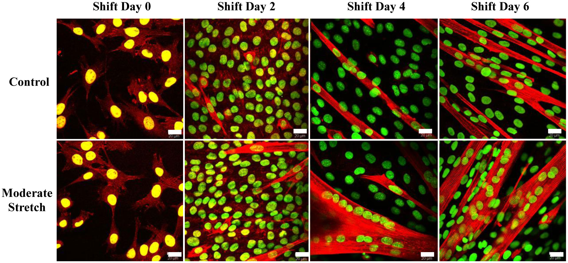
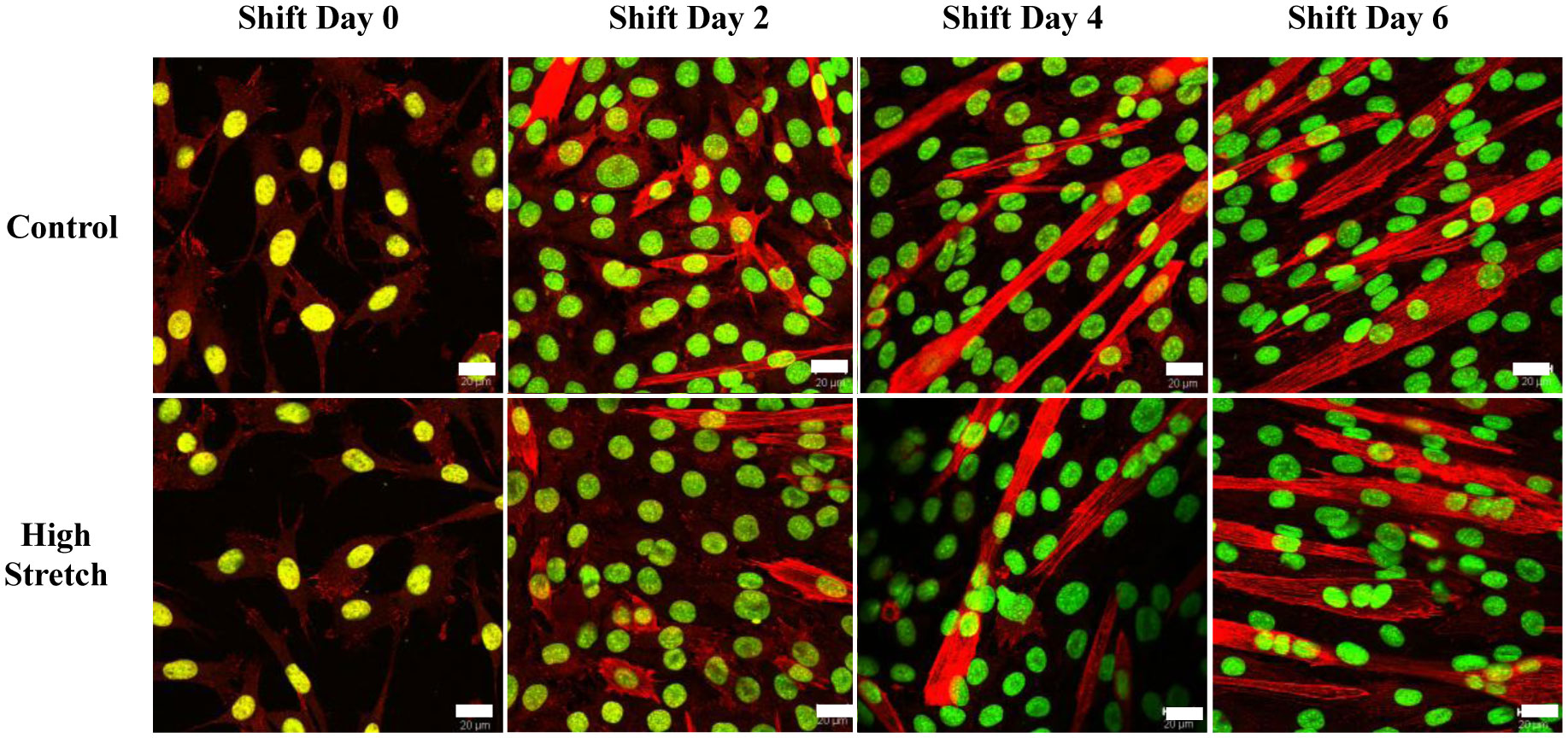
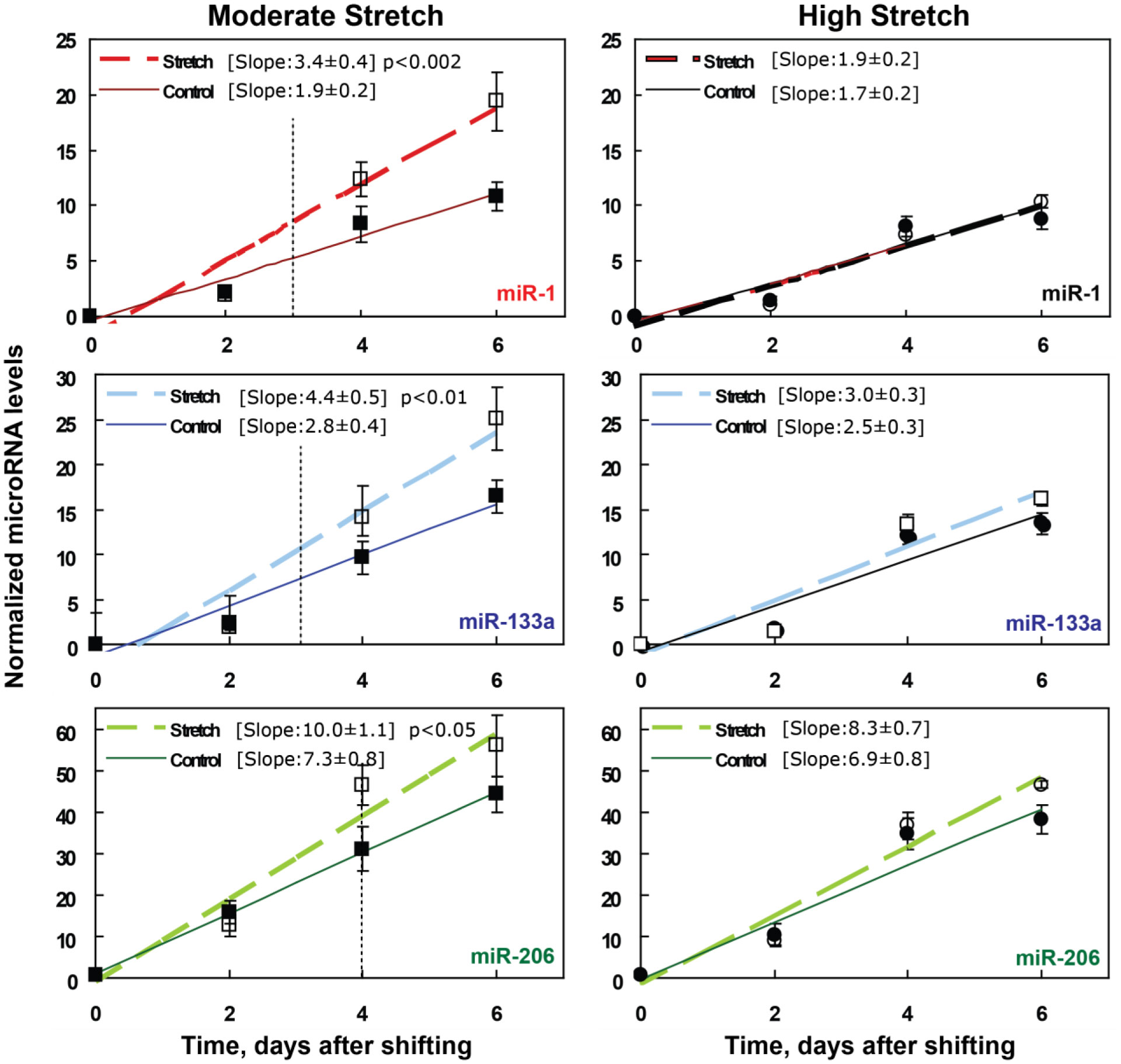
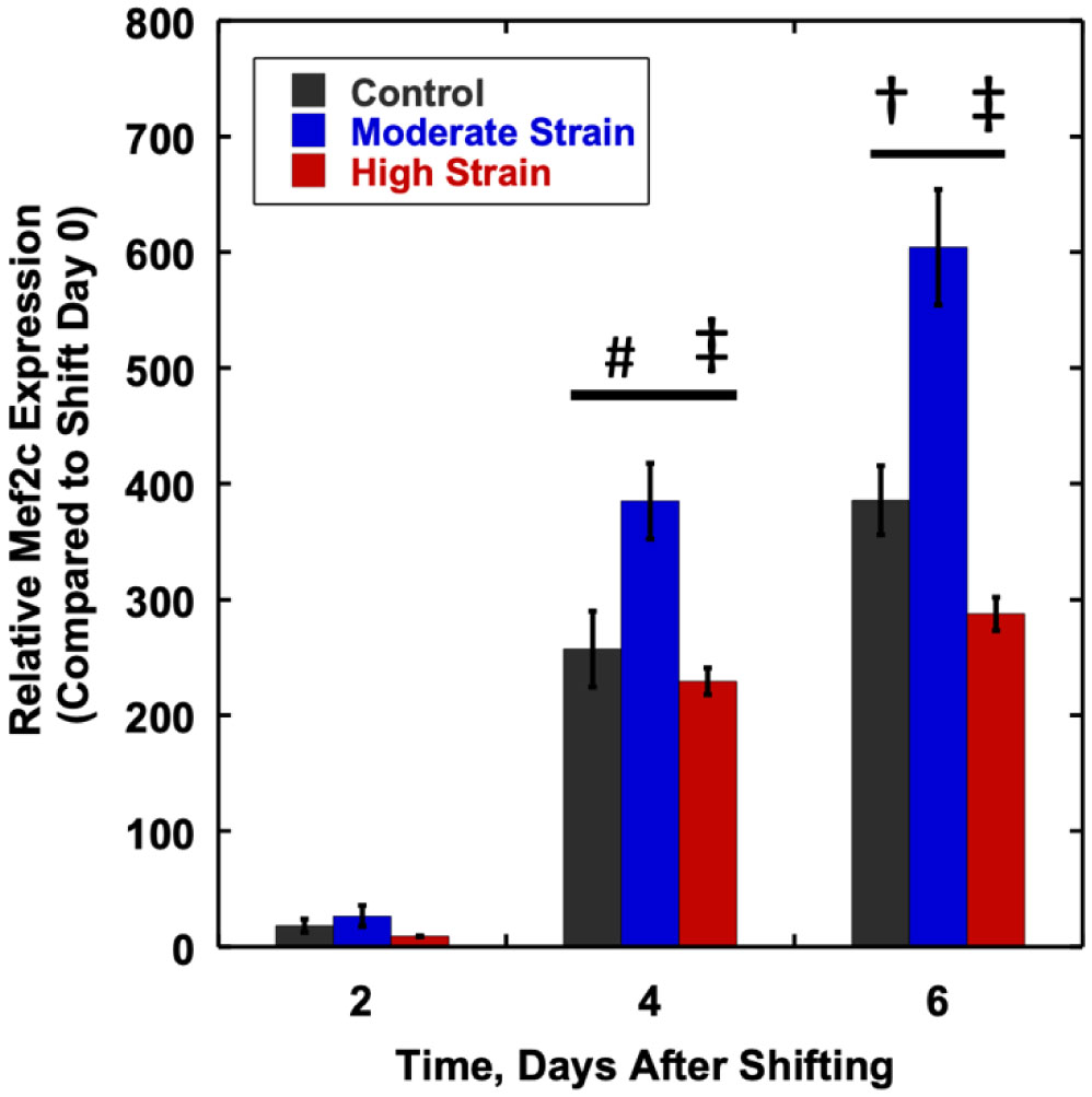
We examined whether mechanical stretch affected expression of muscle-specific microRNAs (miRNAs) that regulate proliferation (miR-133a) or differentiation (miR-1, -206). Real-time quantitative RT-PCR was used to assess miRNA regulation in the murine myoblast cell line C2C12 exposed to stretch regimens that promote either proliferation (high stretch: 17%, 1 Hz) or differentiation (moderate stretch: 10%, 0.5 Hz) after adding media that promotes differentiation. Controls consisted of myoblasts cultured under static conditions. While miRNA expression was not affected by high stretch, a significant effect of stretch (P < 0.05) was seen after 4 days with the moderate stretch regimen. All three microRNAs were upregulated by stretch, with the most significant increase for miR-1. Myoblast maturation was enhanced with a moderate stretch regimen, as assessed by a higher percentage of nuclei in straited fibers and an increase in Mef2c gene expression. Correspondingly, HDAC4 protein expression, a direct target of miR-1 and repressor of Mef2, was decreased with the moderate stretch regimen. Over-expression of miR-1 abrogated the effect of stretch on miR-1, miR-133a and miR-206 levels compared to its negative control but did not alter miR-133a or miR-206 levels. Treatment with an antisense mRNA to miR-1 similarly diminished the stretch-mediated response. Results indicate that the differential response of skeletal myoblasts to moderate and high stretch cyclic stretch regimens is due, in part, to muscle specific miRNA expression.
Citation: Caroline Rhim, William E. Kraus, George A. Truskey. Biomechanical effects on microRNA expression in skeletal muscle differentiation[J]. AIMS Bioengineering, 2020, 7(3): 147-164. doi: 10.3934/bioeng.2020014
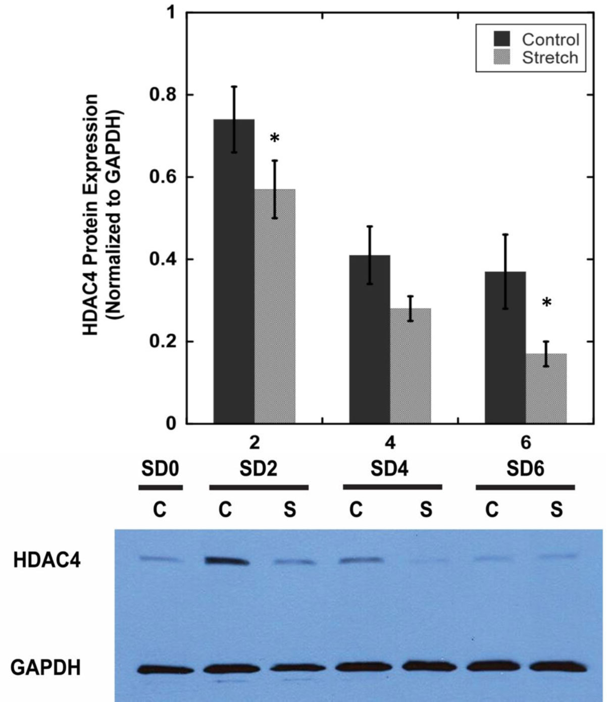
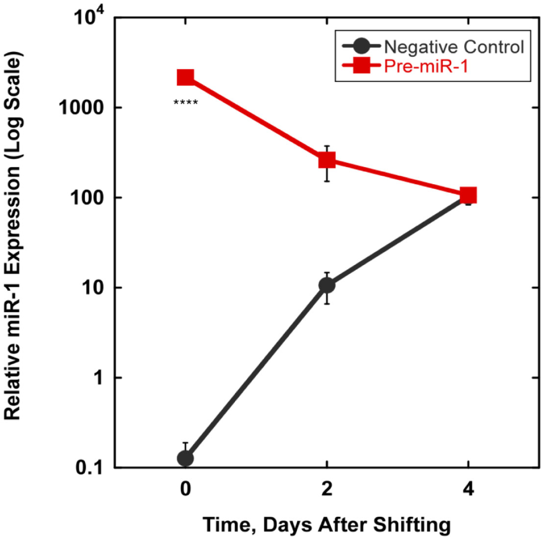
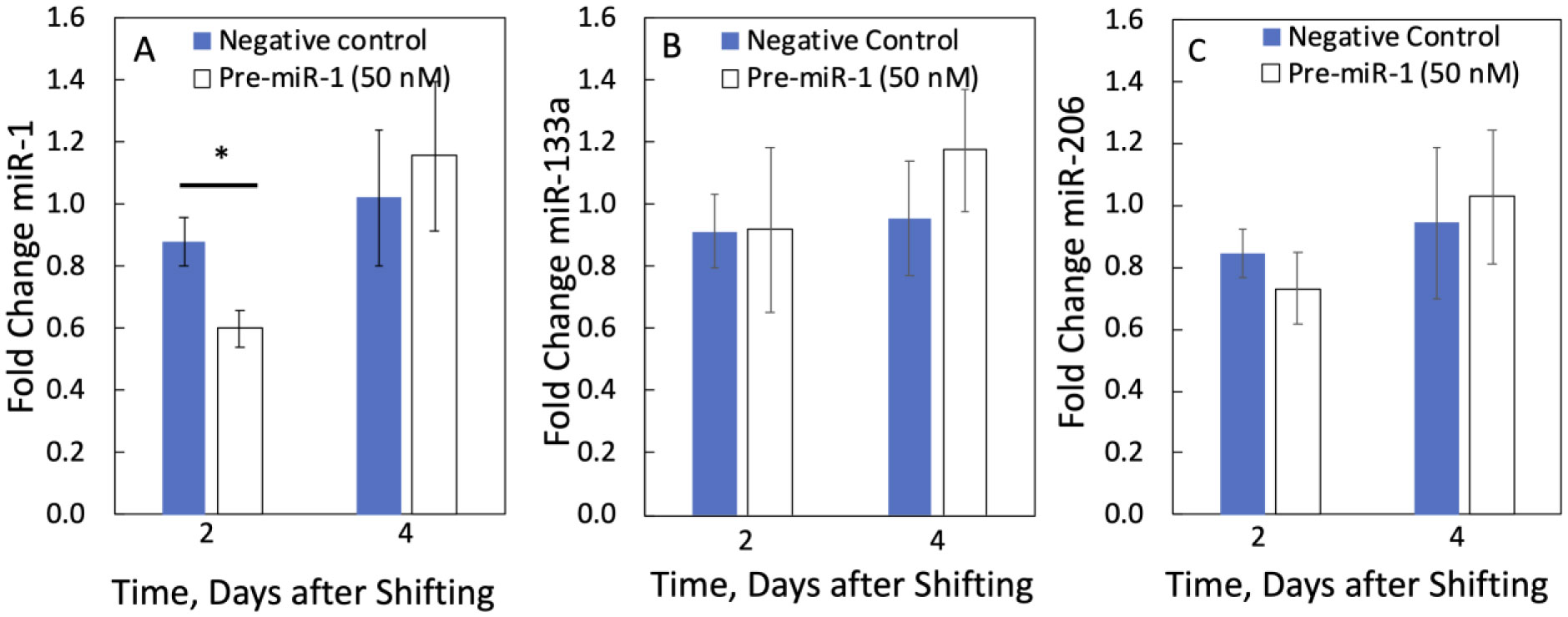
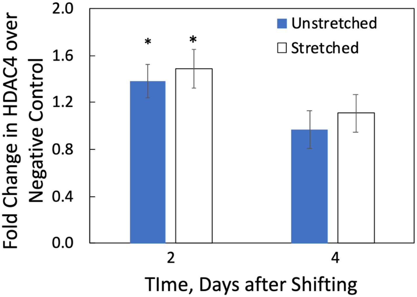
We examined whether mechanical stretch affected expression of muscle-specific microRNAs (miRNAs) that regulate proliferation (miR-133a) or differentiation (miR-1, -206). Real-time quantitative RT-PCR was used to assess miRNA regulation in the murine myoblast cell line C2C12 exposed to stretch regimens that promote either proliferation (high stretch: 17%, 1 Hz) or differentiation (moderate stretch: 10%, 0.5 Hz) after adding media that promotes differentiation. Controls consisted of myoblasts cultured under static conditions. While miRNA expression was not affected by high stretch, a significant effect of stretch (P < 0.05) was seen after 4 days with the moderate stretch regimen. All three microRNAs were upregulated by stretch, with the most significant increase for miR-1. Myoblast maturation was enhanced with a moderate stretch regimen, as assessed by a higher percentage of nuclei in straited fibers and an increase in Mef2c gene expression. Correspondingly, HDAC4 protein expression, a direct target of miR-1 and repressor of Mef2, was decreased with the moderate stretch regimen. Over-expression of miR-1 abrogated the effect of stretch on miR-1, miR-133a and miR-206 levels compared to its negative control but did not alter miR-133a or miR-206 levels. Treatment with an antisense mRNA to miR-1 similarly diminished the stretch-mediated response. Results indicate that the differential response of skeletal myoblasts to moderate and high stretch cyclic stretch regimens is due, in part, to muscle specific miRNA expression.

| [1] | Burkholder TJ, Lieber RL (2001) Sarcomere length operating range of vertebrate muscles during movement. J Exp Biol 204: 1529-1536. |
| [2] |
Zhang SJ, Truskey GA, Kraus WE (2007) Effect of cyclic stretch on β1D-integrin expression and activation of FAK and RhoA. Am J Physiol Cell Physiol 292: C2057-2069. doi: 10.1152/ajpcell.00493.2006

|
| [3] | Vandenburgh HH (1992) Mechanical forces and their second messengers in stimulating cell growth in vitro. Am J Physiol 262: R350-R355. |
| [4] |
Vandenburgh HH, Karlisch P (1989) Longitudinal growth of skeletal myotubes in vitro in a new horizontal mechanical cell stimulator. In Vitro Cell Dev Biol 25: 607-616. doi: 10.1007/BF02623630
|
| [5] |
Kumar A, Murphy R, Robinson P, et al. (2004) Cyclic mechanical strain inhibits skeletal myogenesis through activation of focal adhesion kinase, Rac-1 GTPase, and NF-κB transcription factor. FASEB J 18: 1524-1535. doi: 10.1096/fj.04-2414com
|
| [6] |
Rauch C, Loughna PT (2005) Static stretch promotes MEF2A nuclear translocation and expression of neonatal myosin heavy chain in C2C12 myocytes in a calcineurin- and p38-dependent manner. Am J Physiol Cell Physiol 288: C593-C605. doi: 10.1152/ajpcell.00346.2004
|
| [7] | Kook SH, Lee HJ, Chung WT, et al. (2008) Cyclic mechanical stretch stimulates the proliferation of C2C12 myoblasts and inhibits their differentiation via prolonged activation of p38 MAPK. Mol Cells 25: 479-486. |
| [8] |
Zhao X, Ito A, Kane CD, et al. (2001) The modular nature of histone deacetylase HDAC4 confers phosphorylation-dependent intracellular trafficking. J Biol Chem 276: 35042-35048. doi: 10.1074/jbc.M105086200
|
| [9] |
Zhou X, Richon VM, Wang AH, et al. (2000) Histone deacetylase 4 associates with extracellular signal-regulated kinases 1 and 2, and its cellular localization is regulated by oncogenic Ras. Proc Natl Acad Sci USA 97: 14329-14333. doi: 10.1073/pnas.250494697
|
| [10] |
McKinsey TA, Zhang CL, Lu J, et al. (2000) Signal-dependent nuclear export of a histone deacetylase regulates muscle differentiation. Nature 408: 106-111. doi: 10.1038/35040593
|
| [11] |
Miska EA, Langley E, Wolf D, et al. (2001) Differential localization of HDAC4 orchestrates muscle differentiation. Nucleic Acids Res 29: 3439-3447. doi: 10.1093/nar/29.16.3439
|
| [12] |
Chen JF, Mandel EM, Thomson JM, et al. (2006) The role of microRNA-1 and microRNA-133 in skeletal muscle proliferation and differentiation. Nat Genet 38: 228-233. doi: 10.1038/ng1725
|
| [13] |
Rao PK, Kumar RM, Farkhondeh M, et al. (2006) Myogenic factors that regulate expression of muscle-specific microRNAs. Proc Natl Acad Sci USA 103: 8721-8726. doi: 10.1073/pnas.0602831103
|
| [14] |
Kim HK, Lee YS, Sivaprasad U, et al. (2006) Muscle-specific microRNA miR-206 promotes muscle differentiation. J Cell Biol 174: 677-687. doi: 10.1083/jcb.200603008
|
| [15] |
Baskerville S, Bartel DP (2005) Microarray profiling of microRNAs reveals frequent coexpression with neighboring miRNAs and host genes. RNA 11: 241-247. doi: 10.1261/rna.7240905
|
| [16] |
Wienholds E, Plasterk RHA (2005) MicroRNA function in animal development. FEBS Lett 579: 5911-5922. doi: 10.1016/j.febslet.2005.07.070
|
| [17] |
Lagos-Quintana M, Rauhut R, Yalcin A, et al. (2002) Identification of tissue-specific microRNAs from mouse. Curr Biol 12: 735-739. doi: 10.1016/S0960-9822(02)00809-6
|
| [18] |
Sempere LF, Freemantle S, Pitha-Rowe I, et al. (2004) Expression profiling of mammalian microRNAs uncovers a subset of brain-expressed microRNAs with possible roles in murine and human neuronal differentiation. Genome Biol 5: R13. doi: 10.1186/gb-2004-5-3-r13
|
| [19] |
Ma K, Chan JKL, Zhu G, et al. (2005) Myocyte enhancer factor 2 acetylation by p300 enhances its DNA binding activity, transcriptional activity, and myogenic differentiation. Mol Cell Biol 25: 3575-3582. doi: 10.1128/MCB.25.9.3575-3582.2005
|
| [20] |
Wang DZ (2006) Micro or mega: how important are MicroRNAs in muscle? Cell Cycle 5: 1015-1016. doi: 10.4161/cc.5.10.2742
|
| [21] |
McCarthy JJ (2008) MicroRNA-206: the skeletal muscle-specific myomiR. Biochim Biophys Acta 1779: 682-691. doi: 10.1016/j.bbagrm.2008.03.001
|
| [22] |
Yuasa K, Hagiwara Y, Ando M, et al. (2008) MicroRNA-206 is highly expressed in newly formed muscle fibers: implications regarding potential for muscle regeneration and maturation in muscular dystrophy. Cell Struct Funct 33: 163-169. doi: 10.1247/csf.08022
|
| [23] |
Cheng CS, El-Abd Y, Bui K, et al. (2014) Conditions that promote primary human skeletal myoblast culture and muscle differentiation in vitro. Am J Physiol Cell Physiol 306: C385-C395. doi: 10.1152/ajpcell.00179.2013
|
| [24] |
Kuang W, Tan J, Duan Y, et al. (2009) Cyclic stretch induced miR-146a upregulation delays C2C12 myogenic differentiation through inhibition of Numb. Biochem Bioph Res Commun 378: 259-263. doi: 10.1016/j.bbrc.2008.11.041
|
| [25] |
McCarthy JJ, Esser KA (2007) MicroRNA-1 and microRNA-133a expression are decreased during skeletal muscle hypertrophy. J Appl Physiol 102: 306-313. doi: 10.1152/japplphysiol.00932.2006
|
| [26] |
Care A, Catalucci D, Felicetti F, et al. (2007) MicroRNA-133 controls cardiac hypertrophy. Nat Med 13: 613-618. doi: 10.1038/nm1582
|
| [27] |
Carson JA, Wei L (2000) Integrin signaling's potential for mediating gene expression in hypertrophying skeletal muscle. J Appl Physiol 88: 337-343. doi: 10.1152/jappl.2000.88.1.337
|
| [28] |
Blau HM, Pavlath GK, Hardeman EC, et al. (1985) Plasticity of the differentiated state. Science 230: 758-766. doi: 10.1126/science.2414846
|
| [29] |
Livak KJ, Schmittgen TD (2001) Analysis of relative gene expression data using real-time quantitative PCR and the 2−ΔΔCT method. Methods 25: 402-408. doi: 10.1006/meth.2001.1262
|
| [30] | Zar JH (1999) Biostatistical Analysis. Upper Saddle River NJ: Prentice Hall. |
| [31] |
Feng Y, Cao JH, Li XY, et al. (2011) Inhibition of miR-214 expression represses proliferation and differentiation of C2C12 myoblasts. Cell Biochem Funct 29: 378-383. doi: 10.1002/cbf.1760
|
| [32] |
Wei X, Li H, Zhang B, et al. (2016) miR-378a-3p promotes differentiation and inhibits proliferation of myoblasts by targeting HDAC4 in skeletal muscle development. RNA Biol 13: 1300-1309. doi: 10.1080/15476286.2016.1239008
|
| [33] |
Liu L, Li TM, Liu XR, et al. (2019) MicroRNA-140 inhibits skeletal muscle glycolysis and atrophy in endotoxin-induced sepsis in mice via the WNT signaling pathway. Am J Physiol Cell Physiol 317: C189-C199. doi: 10.1152/ajpcell.00419.2018
|
| [34] |
Su Y, Yu Y, Liu C, et al. (2020) Fate decision of satellite cell differentiation and self-renewal by miR-31-IL34 axis. Cell Death Differ 27: 949-965. doi: 10.1038/s41418-019-0390-x
|
| [35] |
Ge Y, Sun Y, Chen J (2011) IGF-II is regulated by microRNA-125b in skeletal myogenesis. J Cell Biol 192: 69-81. doi: 10.1083/jcb.201007165
|
| [36] |
McCarthy JJ, Esser KA, Andrade FH (2007) MicroRNA-206 is overexpressed in the diaphragm but not the hindlimb muscle of mdx mouse. Am J Physiol Cell Physiol 293: C451-C457. doi: 10.1152/ajpcell.00077.2007
|
| [37] |
Farh KKH, Grimson A, Jan C, et al. (2005) The widespread impact of mammalian MicroRNAs on mRNA repression and evolution. Science 310: 1817-1821. doi: 10.1126/science.1121158
|
| [38] |
Sayed D, Hong C, Chen IY, et al. (2007) MicroRNAs play an essential role in the development of cardiac hypertrophy. Circ Res 100: 416-424. doi: 10.1161/01.RES.0000257913.42552.23
|
| [39] |
Van Rooij E, Olson EN (2007) MicroRNAs: powerful new regualtors of heart disease and provocative therapeutic targets. J Clin Invest 117: 2369-2376. doi: 10.1172/JCI33099
|
| [40] |
Van Rooij E, Sutherland LB, Liu N, et al. (2006) A signature pattern of stress-responsive microRNAs that can evoke cardiac hypertrophy and heart failure. Proc Natl Acad Sci USA 103: 18255-18260. doi: 10.1073/pnas.0608791103
|
| [41] |
Yang B, Lin H, Xiao J, et al. (2007) The muscle-specific microRNA miR-1 regulates cardiac arrhythmogenic potential by targeting GJA1 and KCNJ2. Nat Med 13: 486-491. doi: 10.1038/nm1569
|
| [42] |
Potthoff MJ, Olson EN (2007) MEF2: a central regulator of diverse developmental programs. Development 134: 4131-4140. doi: 10.1242/dev.008367
|
| [43] |
Chan JKL, Sun L, Yang XJ, et al. (2003) Functional characterization of an amino-terminal region of HDAC4 that possesses MEF2 binding and transcriptional repressive activity. J Biol Chem 278: 23515-234521. doi: 10.1074/jbc.M301922200
|
| [44] |
Liu N, Williams AH, Kim Y, et al. (2007) An intragenic MEF2-dependent enhancer directs muscle-specific expression of microRNAs 1 and 133. Proc Natl Acad Sci USA 104: 20844-20849. doi: 10.1073/pnas.0710558105
|
| [45] |
Zhao Y, Samal E, Srivastava D (2005) Serum response factor regulates a muscle-specific microRNA that targets Hand2 during cardiogenesis. Nature 436: 214-220. doi: 10.1038/nature03817
|
| [46] |
Van Rooij E, Liu N, Olson EN (2008) MicroRNAs flex their muscles. Trends Genet 24: 159-166. doi: 10.1016/j.tig.2008.01.007
|
 bioeng-07-03-014-s001.pdf bioeng-07-03-014-s001.pdf |
 |
Figures(8) / Tables(1)

Caroline Rhim, William E. Kraus, George A. Truskey. Biomechanical effects on microRNA expression in skeletal muscle differentiation[J]. AIMS Bioengineering, 2020, 7(3): 147-164. doi: 10.3934/bioeng.2020014


 DownLoad: