Deep neural networks with application in predicting the spread of avian influenza through disease-informed neural networks

Nickson Golooba; Woldegebriel Assefa Woldegerima; Huaiping Zhu; Nickson Golooba; Woldegebriel Assefa Woldegerima; Huaiping Zhu

doi:10.3934/bdia.2025001

Big Data and Information Analytics

2025, Volume 9, 1-28. doi: 10.3934/bdia.2025001

Previous Article Next Article

Research article

Deep neural networks with application in predicting the spread of avian influenza through disease-informed neural networks

Nickson Golooba ¹,
Woldegebriel Assefa Woldegerima ^{2,3
,
,},
Huaiping Zhu ^1,2

1.
Laboratory of Mathematical Parallel Systems (LAMPS), CDM, and OMNI-RÉUNIS, Department of Mathematics and Statistics, York University, Toronto, Canada
2.
Centre for Disease Modeling (CDM), Department of Mathematics and Statistics, York University, Toronto, Canada
3.
Laboratory for Industrial and Applied Mathematics (LIAM), Department of Mathematics and Statistics, York University, Toronto, Canada

Received: 09 December 2024 Revised: 01 February 2025 Accepted: 07 February 2025 Published: 21 March 2025

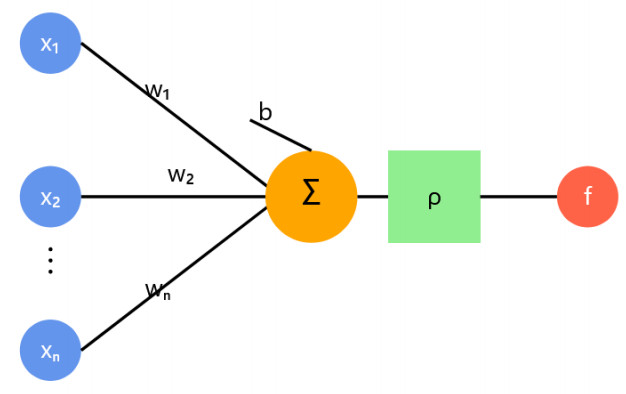
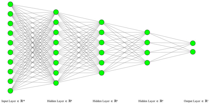
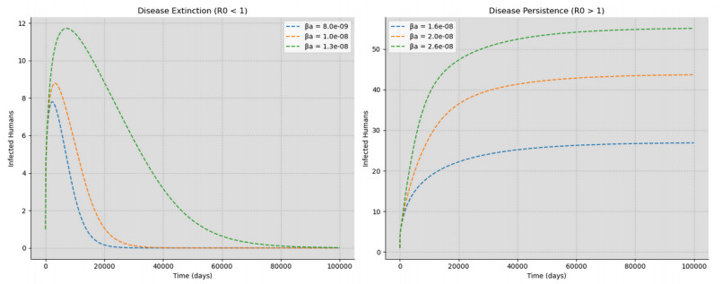
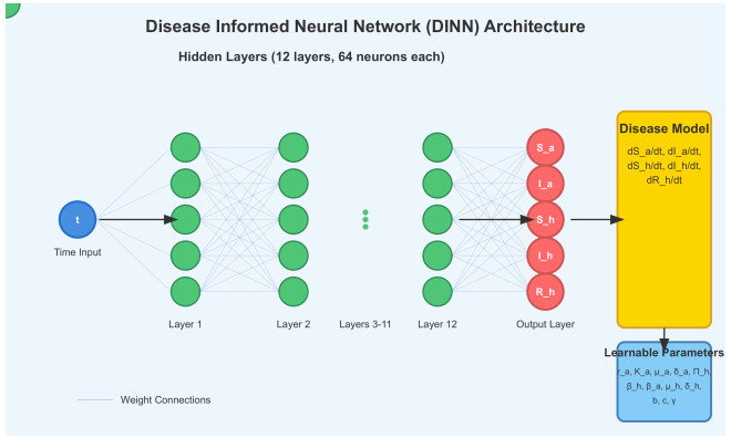
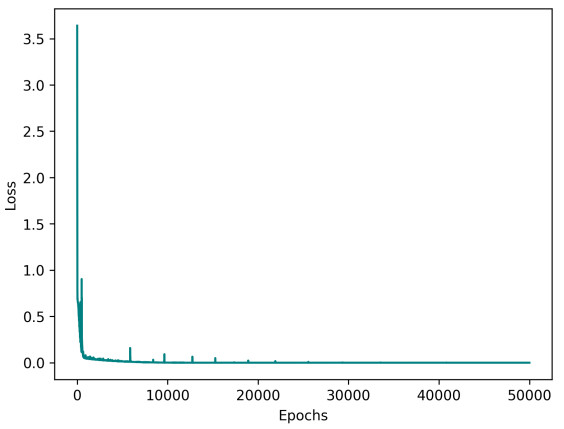
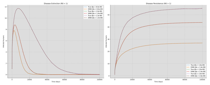
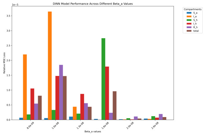
Deep learning has emerged in many fields in recent times where neural networks are used to learn and understand data. This study combined deep learning frameworks with epidemiological models and was aimed specifically at the creation and testing of disease-informed neural networks (DINNs) with a view of modeling the infection dynamics of epidemics. Our research thus trained the DINN on synthetic data derived from a susceptible infected-susceptible infected removed (SI-SIR) model designed for avian influenza and showed the model's accuracy in predicting extinction and persistence conditions. In the method, a twelve hidden layer model was constructed with sixty-four neurons per layer and the rectified linear unit activation function was used. The network was trained to predict the time evolution of five state variables for birds and humans over 50,000 epochs. The overall loss minimized to 0.000006, characterized by a combination of data and physics losses, enabling the DINN to follow the differential equations describing the disease progression.
- disease-informed neural network,
- physics-informed neural networks,
- deep neural networks,
- avian influenza,
- SI-SIR model,
- data and physics loss functions,
- neural network architecture
Citation: Nickson Golooba, Woldegebriel Assefa Woldegerima, Huaiping Zhu. Deep neural networks with application in predicting the spread of avian influenza through disease-informed neural networks[J]. Big Data and Information Analytics, 2025, 9: 1-28. doi: 10.3934/bdia.2025001

Related Papers:

Abstract

Deep learning has emerged in many fields in recent times where neural networks are used to learn and understand data. This study combined deep learning frameworks with epidemiological models and was aimed specifically at the creation and testing of disease-informed neural networks (DINNs) with a view of modeling the infection dynamics of epidemics. Our research thus trained the DINN on synthetic data derived from a susceptible infected-susceptible infected removed (SI-SIR) model designed for avian influenza and showed the model's accuracy in predicting extinction and persistence conditions. In the method, a twelve hidden layer model was constructed with sixty-four neurons per layer and the rectified linear unit activation function was used. The network was trained to predict the time evolution of five state variables for birds and humans over 50,000 epochs. The overall loss minimized to 0.000006, characterized by a combination of data and physics losses, enabling the DINN to follow the differential equations describing the disease progression.

References

[1]	Shaier S, Raissi M, Seshaiyer P, Data-driven approaches for predicting spread of infectious diseases through dinns: Disease informed neural networks. preprint, arXiv: 2110.05445. https://doi.org/10.48550/arXiv.2110.05445
[2]	Lichtner-Bajjaoui A, A Mathematical Introduction to Neural Networks. Master's thesis, Universitat de Barcelona, 2021.
[3]	McCulloch WS, Pitts W, (1943) A logical calculus of the ideas immanent in nervous activity. Bull Math Biophys 5: 115–133. https://doi.org/10.1007/BF02478259 doi: 10.1007/BF02478259
[4]	Kutyniok G, The mathematics of artificial intelligence. preprint, arXiv: 2203.08890. https://doi.org/10.48550/arXiv.2203.08890
[5]	Galván E, Mooney P, (2021) Neuroevolution in deep neural networks: Current trends and future challenges. IEEE Trans Artif Intell 2: 476–493. https://doi.org/10.1109/TAI.2021.3067574 doi: 10.1109/TAI.2021.3067574
[6]	Hethcote HW, (2000) The mathematics of infectious diseases. SIAM Rev 42: 599–653. https://doi.org/10.1137/S0036144500371907 doi: 10.1137/S0036144500371907
[7]	Brauer F, Castillo-Chavez C, (2012) Mathematical Models in Population Biology and Epidemiology, 2 Eds., New York: Springer. https://doi.org/10.1007/978-1-4614-1686-9
[8]	Brauer F, Castillo-Chavez C, Feng Z, (2019) Mathematical Models in Epidemiology, New York: Springer. https://doi.org/10.1007/978-1-4939-9828-9
[9]	Holzinger A, Biemann C, Pattichis CS, Kell DB, What do we need to build explainable ai systems for the medical domain?. preprint, arXiv: 1712.09923. https://doi.org/10.48550/arXiv.1712.09923
[10]	Liu S, Ruan S, Zhang X, (2017) Nonlinear dynamics of avian influenza epidemic models. Math Biosci 283: 118–135. https://doi.org/10.1016/j.mbs.2016.11.014 doi: 10.1016/j.mbs.2016.11.014
[11]	Yu X, Ma Y, (2022) An avian influenza model with nonlinear incidence and recovery rates in deterministic and stochastic environments. Nonlinear Dyn 108: 4611–4628. https://doi.org/10.1007/s11071-022-07422-6 doi: 10.1007/s11071-022-07422-6
[12]	Yang S, Santillana M, Kou SC, (2015) Accurate estimation of influenza epidemics using google search data via ARGO, In: Proceedings of the National Academy of Sciences, 112: 14473–14478. https://doi.org/10.1073/pnas.1515373112
[13]	Wiens J, Shenoy ES, (2018) Machine learning for healthcare: On the verge of a major shift in healthcare epidemiology. Clin Infect Dis 66: 149–153. https://doi.org/10.1093/cid/cix731 doi: 10.1093/cid/cix731
[14]	Raissi M, Perdikaris P, Karniadakis GE, (2019) Physics-informed neural networks: A deep learning framework for solving forward and inverse problems involving nonlinear partial differential equations. J Comput Phys 378: 686–707. https://doi.org/10.1016/j.jcp.2018.10.045 doi: 10.1016/j.jcp.2018.10.045
[15]	Nguyen L, Raissi M, Seshaiyer P, (2022) Modeling, analysis and physics informed neural network approaches for studying the dynamics of COVID-19 involving human-human and human-pathogen interaction. Comput Math Biophys 10: 1–17. https://doi.org/10.1515/cmb-2022-0001 doi: 10.1515/cmb-2022-0001
[16]	Ning X, Jia L, Wei Y, Li XA, Chen F, (2023) Epi-DNNs: Epidemiological priors informed deep neural networks for modeling COVID-19 dynamics. Comput Biol Med 158: 106693. https://doi.org/10.1016/j.compbiomed.2023.106693 doi: 10.1016/j.compbiomed.2023.106693
[17]	Kutyniok G, (2023) An introduction to the mathematics of deep learning, In: European Congress of Mathematics, 73–91. https://doi.org/10.4171/8ECM/30
[18]	Goodfellow I, Bengio Y, Courville A, (2016) Deep learning, MIT Press. https://doi.org/10.4258/hir.2016.22.4.351
[19]	Rumelhart DE, Hinton GE, Williams RJ, (1986) Learning representations by back-propagating errors. Nature 323: 533–536. https://doi.org/10.1038/323533a0 doi: 10.1038/323533a0
[20]	Glorot X, Bordes A, Bengio Y, (2011) Deep sparse rectifier neural networks, In Proceedings of the Fourteenth International Conference on Artificial Intelligence and Statistics, 315–323.
[21]	Lenail A, (2019) NN-SVG: Publication-ready neural network architecture schematics. J Open Source Softw 4: 747. https://doi.org/10.21105/joss.00747. doi: 10.21105/joss.00747
[22]	Tieleman T, (2012) Lecture 6.5-rmsprop: Divide the gradient by a running average of its recent magnitude. COURSERA Neural Networks Mach Learn 4: 26.
[23]	Kingma DP, Ba J, Adam: A method for stochastic optimization. preprint, arXiv: 1412.6980. https://doi.org/10.48550/arXiv.1412.6980
[24]	Hornik K, (1991) Approximation capabilities of multilayer feedforward networks. Neural Networks 4: 251–257. https://doi.org/10.1016/0893-6080(91)90009-T doi: 10.1016/0893-6080(91)90009-T
[25]	Hornik K, Stinchcombe M, White H, (1989) Multilayer feedforward networks are universal approximators. Neural Networks 2: 359–366. https://doi.org/10.1016/0893-6080(89)90020-8 doi: 10.1016/0893-6080(89)90020-8
[26]	Funahashi KI, (1989) On the approximate realization of continuous mappings by neural networks. Neural networks 2: 183–192. https://doi.org/10.1016/0893-6080(89)90003-8 doi: 10.1016/0893-6080(89)90003-8
[27]	Shao W, Li X, Goraya MU, Wang S, Chen JL, (2017) Evolution of influenza a virus by mutation and re-assortment. Int J Mol Sci 18: 1650. https://doi.org/10.3390/ijms18081650 doi: 10.3390/ijms18081650
[28]	Peiris JM, De Jong MD, Guan Y, (2007) Avian influenza virus (H5N1): A threat to human health. Clin Microbiol Rev 20: 243–267. https://doi.org/10.1128/cmr.00037-06 doi: 10.1128/cmr.00037-06
[29]	Alexander DJ, (2007) An overview of the epidemiology of avian influenza. Vaccine 25: 5637–5644. https://doi.org/10.1016/j.vaccine.2006.10.051 doi: 10.1016/j.vaccine.2006.10.051
[30]	Gao R, Cao B, Hu Y, Feng Z, Wang D, Hu W, et al. (2013) Human infection with a novel avian-origin influenza A (H7N9) virus. N Engl J Med, 368: 1888–1897. https://doi.org/10.1056/NEJMoa1304459 doi: 10.1056/NEJMoa1304459
[31]	Centers for Disease Control and Prevention, Avian Influenza in Mammals, 2024. Available from: https://www.cdc.gov/bird-flu/situation-summary/mammals.html.
[32]	USDA, USDA, FDA and CDC Share Update on HPAI Detections in Dairy Cattle, 2024. Available from: https://www.aphis.usda.gov/news/agency-announcements/usda-fda-cdc-share-update-hpai-detections-dairy-cattle.
[33]	Government of Canada, The Government of Canada provides an update on Highly Pathogenic Avian Influenza, 2024. Available from: https://www.canada.ca/en/food-inspection-agency/news/2024/05/the-government-of-canada-provides-an-update-on-the-highly-pathogenic-avian-influenza.html.
[34]	Government of Canada, Animals susceptible to H5N1 highly pathogenic avian influenza (HPAI), 2024. Available from: https://inspection.canada.ca/en/animal-health/terrestrial-animals/diseases/reportable/avian-influenza/animals-susceptible-h5n1-hpai.
[35]	Peng L, Yang W, Zhang D, Zhuge C, Hong L, Epidemic analysis of COVID-19 in China by dynamical modeling. preprint, arXiv: 2002.06563. https://doi.org/10.48550/arXiv.2002.06563
[36]	Ning X, Guan J, Li XA, Wei Y, Chen F, (2023) Physics-informed neural networks integrating compartmental model for analyzing COVID-19 transmission dynamics. Viruses 15: 1749. https://doi.org/10.3390/v15081749 doi: 10.3390/v15081749
[37]	Yang Z, Zeng Z, Wang K, Wong SS, Liang W, Zanin M, et al. (2020) Modified SEIR and AI prediction of the epidemics trend of COVID-19 in China under public health interventions. J Thorac Dis, 12: 165. https://doi.org/10.21037/jtd.2020.02.64 doi: 10.21037/jtd.2020.02.64

Reader Comments

Your name:*

Email:*
© 2025 the Author(s), licensee AIMS Press. This is an open access article distributed under the terms of the Creative Commons Attribution License (http://creativecommons.org/licenses/by/4.0)