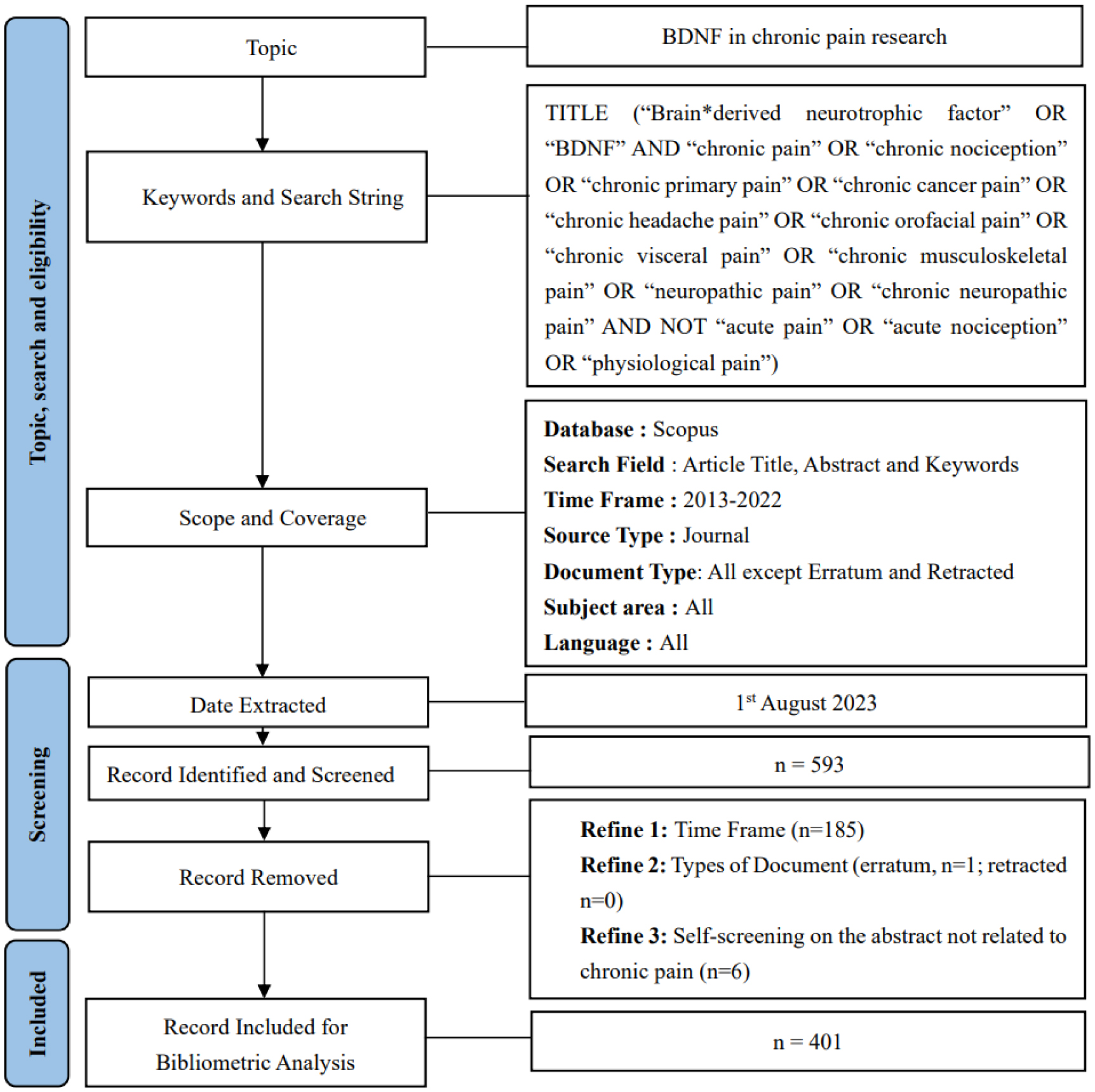
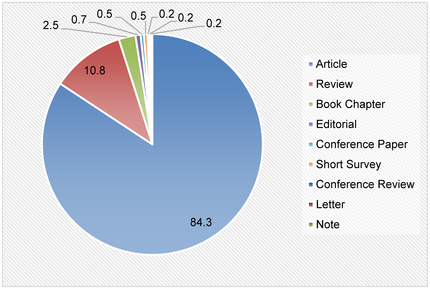
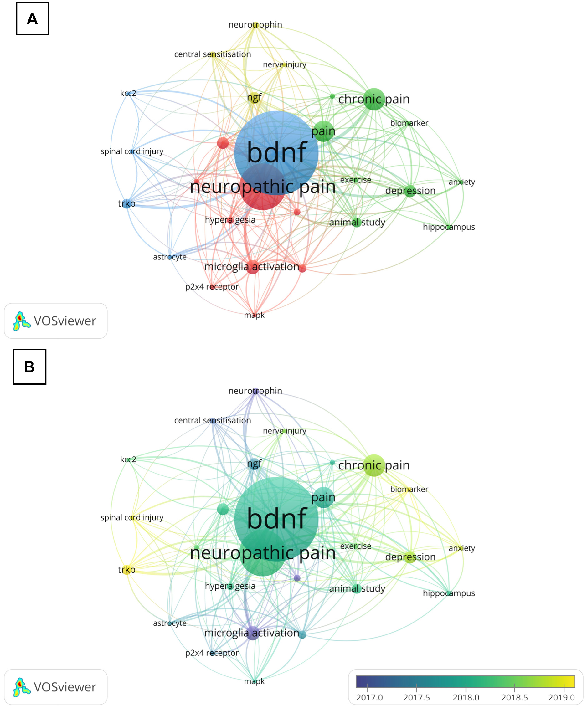
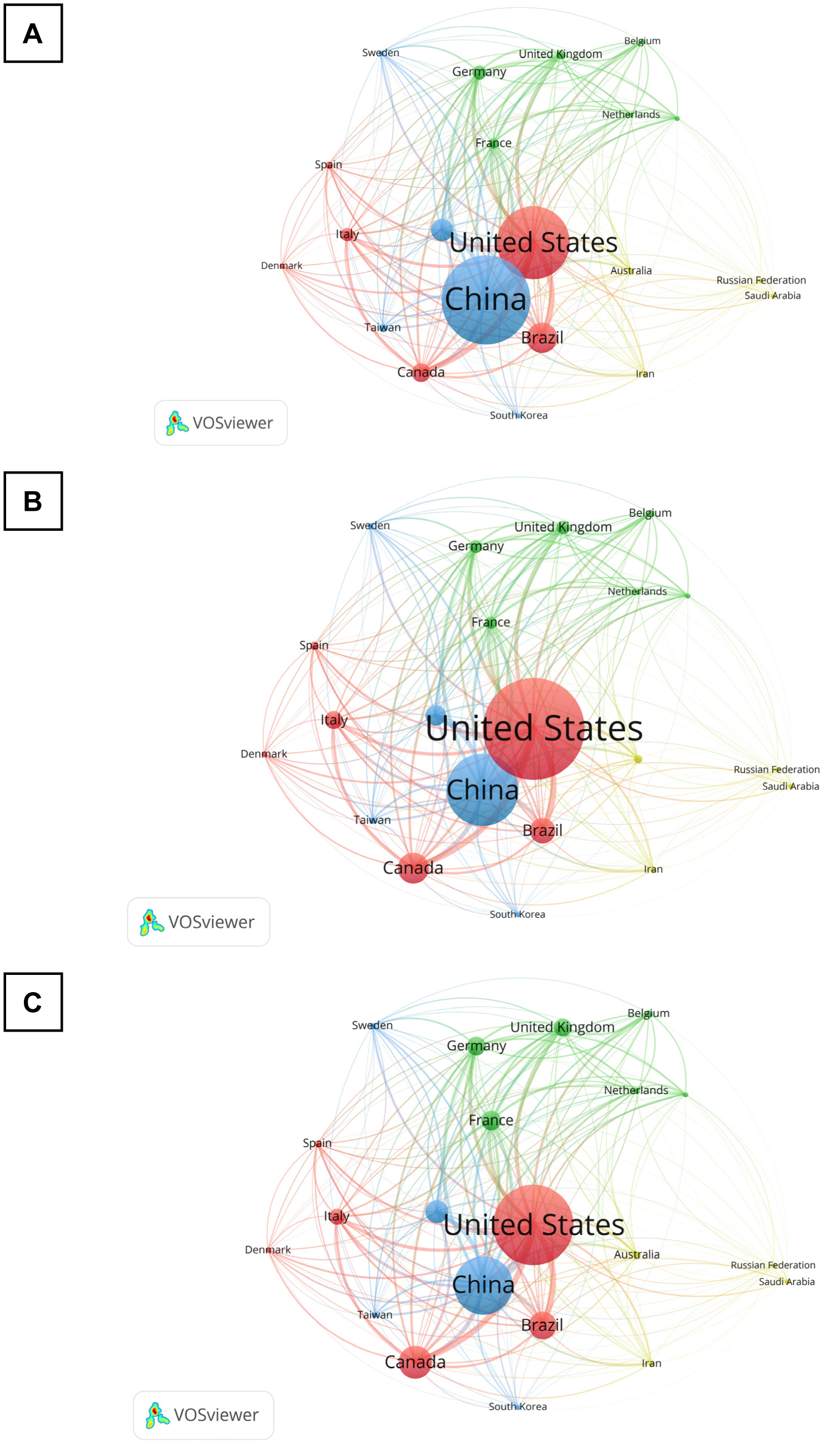
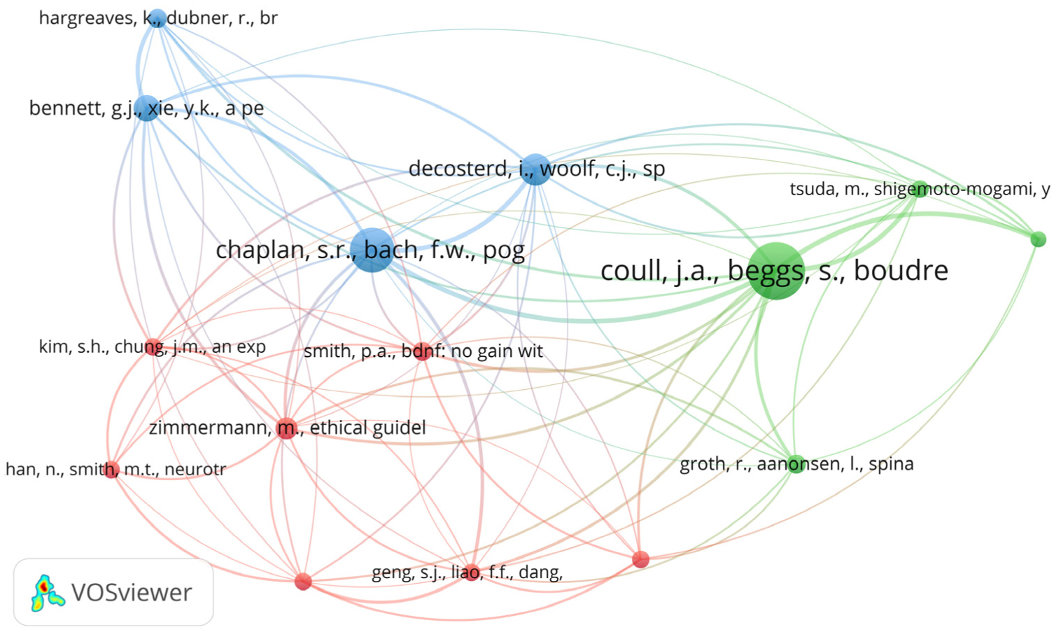
Chronic pain research, with a specific focus on the brain-derived neurotrophic factor (BDNF), has made impressive progress in the past decade, as evident in the improved research quality and increased publications. To better understand this evolving landscape, a quantitative approach is needed. The main aim of this study is to identify the hotspots and trends of BDNF in chronic pain research. We screened relevant publications from 2013 to 2022 in the Scopus database using specific search subject terms. A total of 401 documents were selected for further analysis. We utilized several tools, including Microsoft Excel, Harzing's Publish or Perish, and VOSViewer, to perform a frequency analysis, citation metrics, and visualization, respectively. Key indicators that were examined included publication growth, keyword analyses, topmost influential articles and journals, networking by countries and co-citation of cited references. Notably, there was a persistent publication growth between 2015 and 2021. “Neuropathic pain” emerged as a prominent keyword in 2018, alongside “microglia” and “depression”. The journal Pain® was the most impactful journal that published BDNF and chronic pain research, while the most influential publications came from open-access reviews and original articles. China was the leading contributor, followed by the United States (US), and maintained a leadership position in the total number of publications and collaborations. In conclusion, this study provides a comprehensive list of the most influential publications on BDNF in chronic pain research, thereby aiding in the understanding of academic concerns, research hotspots, and global trends in this specialized field.
Citation: Che Aishah Nazariah Ismail, Rahimah Zakaria, Khairunnuur Fairuz Azman, Nazlahshaniza Shafin, Noor Azlina Abu Bakar. Brain-derived neurotrophic factor (BDNF) in chronic pain research: A decade of bibliometric analysis and network visualization[J]. AIMS Neuroscience, 2024, 11(1): 1-24. doi: 10.3934/Neuroscience.2024001
Chronic pain research, with a specific focus on the brain-derived neurotrophic factor (BDNF), has made impressive progress in the past decade, as evident in the improved research quality and increased publications. To better understand this evolving landscape, a quantitative approach is needed. The main aim of this study is to identify the hotspots and trends of BDNF in chronic pain research. We screened relevant publications from 2013 to 2022 in the Scopus database using specific search subject terms. A total of 401 documents were selected for further analysis. We utilized several tools, including Microsoft Excel, Harzing's Publish or Perish, and VOSViewer, to perform a frequency analysis, citation metrics, and visualization, respectively. Key indicators that were examined included publication growth, keyword analyses, topmost influential articles and journals, networking by countries and co-citation of cited references. Notably, there was a persistent publication growth between 2015 and 2021. “Neuropathic pain” emerged as a prominent keyword in 2018, alongside “microglia” and “depression”. The journal Pain® was the most impactful journal that published BDNF and chronic pain research, while the most influential publications came from open-access reviews and original articles. China was the leading contributor, followed by the United States (US), and maintained a leadership position in the total number of publications and collaborations. In conclusion, this study provides a comprehensive list of the most influential publications on BDNF in chronic pain research, thereby aiding in the understanding of academic concerns, research hotspots, and global trends in this specialized field.

| [1] |
Şentürk İA, Şentürk E, Üstün I, et al. (2023) High-impact chronic pain: evaluation of risk factors and predictors. Korean J Pain 36: 84-97. https://doi.org/10.3344/kjp.22357 
|
| [2] |
Hutton D, Mustafa A, Patil S, et al. (2023) The burden of Chronic Pelvic Pain (CPP): Costs and quality of life of women and men with CPP treated in outpatient referral centers. Plos One 18: e0269828. https://doi.org/10.1371/journal.pone.0269828
|
| [3] |
Nahin RL, Feinberg T, Kapos FP, et al. (2023) Estimated Rates of Incident and Persistent Chronic Pain Among US Adults, 2019-2020. JAMA Netw Open 6: e2313563. https://doi.org/10.1001/jamanetworkopen.2023.13563
|
| [4] |
Collier R (2018) A short history of pain management. Can Med Assoc J 190: E26-E27. https://doi.org/10.1503/cmaj.109-5523
|
| [5] |
Ikeda K, Hazama K, Itano Y, et al. (2020) Development of a novel analgesic for neuropathic pain targeting brain-derived neurotrophic factor. Biochem Biophys Res Commun 531: 390-395. https://doi.org/10.1016/j.bbrc.2020.07.109
|
| [6] |
Bathina S, Das UN (2015) Brain-derived neurotrophic factor and its clinical implications. Arch Med Sci 11: 1164-1178. https://doi.org/10.5114/aoms.2015.56342
|
| [7] |
Sikandar S, Minett MS, Millet Q, et al. (2018) Brain-derived neurotrophic factor derived from sensory neurons plays a critical role in chronic pain. Brain 141: 1028-1039. https://doi.org/10.1093/brain/awy009
|
| [8] |
Sosanya NM, Garza TH, Stacey W, et al. (2019) Involvement of brain-derived neurotrophic factor (BDNF) in chronic intermittent stress-induced enhanced mechanical allodynia in a rat model of burn pain. BMC Neurosci 20: 1-18. https://doi.org/10.1186/s12868-019-0500-1
|
| [9] |
Eaton MJ, Blits B, Ruitenberg MJ, et al. (2002) Amelioration of chronic neuropathic pain after partial nerve injury by adeno-associated viral (AAV) vector-mediated over-expression of BDNF in the rat spinal cord. Gene Ther 9: 1387-1395. https://doi.org/10.1038/sj.gt.3301814
|
| [10] |
Thomas Cheng H (2010) Spinal cord mechanisms of chronic pain and clinical implications. Curr Pain Headache Rep 14: 213-220. https://doi.org/10.1007/s11916-010-0111-0
|
| [11] |
Ding X, Cai J, Li S, et al. (2015) BDNF contributes to the development of neuropathic pain by induction of spinal long-term potentiation via SHP2 associated GluN2B-containing NMDA receptors activation in rats with spinal nerve ligation. Neurobiol Dis 73: 428-451. https://doi.org/10.1016/j.nbd.2014.10.025
|
| [12] |
Zhou LJ, Yang T, Wei X, et al. (2011) Brain-derived neurotrophic factor contributes to spinal long-term potentiation and mechanical hypersensitivity by activation of spinal microglia in rat. Brain Behav Immun 25: 322-334. https://doi.org/10.1016/j.bbi.2010.09.025
|
| [13] |
Zhou W, Xie Z, Li C, et al. (2021) Driving effect of BDNF in the spinal dorsal horn on neuropathic pain. Neurosci Lett 756: 135965. https://doi.org/10.1016/j.neulet.2021.135965
|
| [14] |
Coull JAM, Beggs S, Boudreau D, et al. (2005) BDNF from microglia causes the shift in neuronal anion gradient underlying neuropathic pain. Nature 438: 1017-1021. https://doi.org/10.1038/nature04223
|
| [15] |
Thakkar B, Acevedo EO (2023) BDNF as a biomarker for neuropathic pain: Consideration of mechanisms of action and associated measurement challenges. Brain Behav 13: e2903. https://doi.org/10.1002/brb3.2903
|
| [16] |
Cao T, Matyas JJ, Renn CL, et al. (2020) Function and mechanisms of truncated BDNF receptor TrkB.T1 in neuropathic pain. Cells 9: 1194. https://doi.org/10.3390/cells9051194
|
| [17] |
He T, Wu Z, Zhang X, et al. (2022) A bibliometric analysis of research on the role of BDNF in depression and treatment. Biomolecules 12: 1464. https://doi.org/10.3390/biom12101464
|
| [18] |
Abramo G, D'Angelo CA, Viel F (2011) The field-standardized average impact of national research systems compared to world average: the case of Italy. Scientometrics 88: 599-615. https://doi.org/10.1007/s11192-011-0406-x
|
| [19] |
Ahmad R, Azman KF, Yahaya R, et al. (2023) Brain-derived neurotrophic factor (BDNF) in schizophrenia research: a quantitative review and future directions. AIMS Neurosci 10: 5-32. https://doi.org/10.3934/Neuroscience.2023002
|
| [20] |
Fei X, Wang S, Li J, et al. (2022) Bibliometric analysis of research on Alzheimer's disease and non-coding RNAs: opportunities and challenges. Front Aging Neurosci 14: 1037068. https://doi.org/10.3389/fnagi.2022.1037068
|
| [21] | Martínez-Ezquerro JD, Michán L, Rosas-Vargas H (2016) Bibliometric analysis of the BDNF Val66Met polymorphism based on Web of Science, Pubmed, and Scopus databases. Paper presented at: 29th National Congress of Biochemistry, Mexican Society of Biochemistry (SMB) 2012 . https://doi.org/10.7490/f1000research.1113470.1 |
| [22] |
Othman Z, Abdul Halim AS, Azman KF, et al. (2022) Profiling the research landscape on cognitive aging: A bibliometric analysis and network visualization. Front Aging Neurosci 14: 876159. https://doi.org/10.3389/fnagi.2022.876159
|
| [23] |
Zhu J, Liu W (2020) A tale of two databases: The use of Web of Science and Scopus in academic papers. Scientometrics 123: 321-335. https://doi.org/10.1007/s11192-020-03387-8
|
| [24] |
Pranckutė R (2021) Web of Science (WoS) and Scopus: The titans of bibliographic information in today's academic world. Publications 9: 12. https://doi.org/10.3390/publications9010012
|
| [25] |
Ferrini F, De Koninck Y (2013) Microglia control neuronal network excitability via BDNF signaling. Neural Plast 2013: 429815. https://doi.org/10.1155/2013/429815
|
| [26] |
Liu Y, Zhou L-J, Wang J, et al. (2017) TNF-α differentially regulates synaptic plasticity in the hippocampus and spinal cord by microglia-dependent mechanisms after peripheral nerve injury. J Neurosci 37: 871-881. https://doi.org/10.1523/JNEUROSCI.2235-16.2016
|
| [27] |
Gomes C, Ferreira R, George J, et al. (2013) Activation of microglial cells triggers a release of brain-derived neurotrophic factor (BDNF) inducing their proliferation in an adenosine A2A receptor-dependent manner: A2A receptor blockade prevents BDNF release and proliferation of microglia. J Neuroinflamm 10: 1-13. https://doi.org/10.1186/1742-2094-10-16
|
| [28] |
Taves S, Berta T, Chen G, et al. (2013) Microglia and spinal cord synaptic plasticity in persistent pain. Neural Plast 2013: 753656. https://doi.org/10.1155/2013/753656
|
| [29] |
Yalcin I, Barthas F, Barrot M (2014) Emotional consequences of neuropathic pain: insight from preclinical studies. Neurosci Biobehav Rev 47: 154-164. https://doi.org/10.1016/j.neubiorev.2014.08.002
|
| [30] |
Taylor AMW, Castonguay A, Taylor AJ, et al. (2015) Microglia disrupt mesolimbic reward circuitry in chronic pain. J Neurosci 35: 8442-8450. https://doi.org/10.1523/JNEUROSCI.4036-14.2015
|
| [31] |
Khan N, Smith MT (2015) Neurotrophins and neuropathic pain: role in pathobiology. Molecules 20: 10657-10688. https://doi.org/10.3390/molecules200610657
|
| [32] |
Nijs J, Meeus M, Versijpt J, et al. (2015) Brain-derived neurotrophic factor as a driving force behind neuroplasticity in neuropathic and central sensitization pain: a new therapeutic target?. Expert Opin Ther Targets 19: 565-576. https://doi.org/10.1517/14728222.2014.994506
|
| [33] |
Zhou L-J, Peng J, Xu Y-N, et al. (2019) Microglia are indispensable for synaptic plasticity in the spinal dorsal horn and chronic pain. Cell Rep 27: 3844-3859. https://doi.org/10.1016/j.celrep.2019.05.087
|
| [34] |
Richner M, Ulrichsen M, Elmegaard SL, et al. (2014) Peripheral nerve injury modulates neurotrophin signaling in the peripheral and central nervous system. Mol Neurobiol 50: 945-970. https://doi.org/10.1007/s12035-014-8706-9
|
| [35] |
Chaplan SR, Bach FW, Pogrel JW, et al. (1994) Quantitative assessment of tactile allodynia in the rat paw. J Neurosci Methods 53: 55-63. https://doi.org/10.1016/0165-0270(94)90144-9
|
| [36] |
Decostered I, Woolf CJ (2000) Spared nerve injury: an animal model of persistent peripheral neuropathic pain. Pain 87: 149-158. https://doi.org/10.1016/S0304-3959(00)00276-1
|
| [37] |
Bennett GJ, Xie Y-K (1988) A peripheral mononeuropathy in rat that produces disorders of pain sensation like those seen in man. Pain 33: 87-107. https://doi.org/10.1016/0304-3959(88)90209-6
|
| [38] | Ribeiro VGC, Lacerda ACR, Santos JM, et al. (2021) Efficacy of whole-body vibration training on brain-derived neurotrophic factor, clinical and functional outcomes, and quality of life in women with fibromyalgia syndrome: a randomized controlled trial. J Healthc Eng 2021: 7593802. https://doi.org/10.1155/2021/7593802 |
| [39] |
Sheng J, Liu S, Wang Y, et al. (2017) The link between depression and chronic pain: neural mechanisms in the brain. Neural Plast 2017: 9724371. https://doi.org/10.1155/2017/9724371
|
| [40] |
Zhang S-B, Zhao G-H, Lv T-R, et al. (2023) Bibliometric and visual analysis of microglia-related neuropathic pain from 2000 to 2021. Front Mol Neurosci 16: 1142852. https://doi.org/10.3389/fnmol.2023.1142852
|
| [41] |
Du H, Wu D, Zhong S, et al. (2022) miR-106b-5p attenuates neuropathic pain by regulating the P2x4 receptor in the spinal cord in mice. J Mol Neurosci 72: 1764-1778. https://doi.org/10.1007/s12031-022-02011-z
|
| [42] |
Kohno K, Tsuda M (2021) Role of microglia and P2X4 receptors in chronic pain. Pain Rep 6: e864. https://doi.org/10.1097/PR9.0000000000000864
|
| [43] | Biagioli M, Lippman A (2020) Gaming the metrics: Misconduct and manipulation in academic research. London: MIT Press 1-21. |
| [44] |
Caon M, Trapp J, Baldock C (2020) Citations are a good way to determine the quality of research. Phys Eng Sci Med 43: 1145-1148. https://doi.org/10.1007/s13246-020-00941-9
|
| [45] |
Chuang K-Y, Ho Y-S (2014) A bibliometric analysis on top-cited articles in pain research. Pain Med 15: 732-744. https://doi.org/10.1111/pme.12308
|
| [46] |
Thelwall M, Sud P (2022) Scopus 1900–2020: Growth in articles, abstracts, countries, fields, and journals. Quant Sci 3: 37-50. https://doi.org/10.1162/qss_a_00177
|
| [47] |
Xiong H-Y, Liu H, Wang X-Q (2021) Top 100 most-cited papers in neuropathic pain from 2000 to 2020: a bibliometric study. Front Neurol 12: 765193. https://doi.org/10.3389/fneur.2021.765193
|
| [48] |
Chou C-Y, Chew SSL, Patel DV, et al. (2009) Publication and citation analysis of the Australian and New Zealand Journal of Ophthalmology and Clinical and Experimental Ophthalmology over a 10-year period: the evolution of an ophthalmology journal. Clin Experiment Ophthalmol 37: 868-873. https://doi.org/10.1111/j.1442-9071.2009.02191.x
|
| [49] |
Li X, Zhu W, Li J, et al. (2021) Prevalence and characteristics of chronic Pain in the Chinese community-dwelling elderly: a cross-sectional study. BMC Geriatr 21: 1-10. https://doi.org/10.1186/s12877-021-02432-2
|
| [50] | Surwase G, Saga A, Kadermani BS, et al. (2011) Co-citation analysis: An overview. In: Paper Presented at: Beyond Librarianship: Creativity, Innovation and Discovery, Mumbai (India), 16–17 September 2011 . |
| [51] |
Argüelles JC, Argüelles-Prieto R (2019) The impact factor: implications for research policy, editorial rules and scholarly reputation. FEMS Microbiol Lett 366: fnz132. https://doi.org/10.1093/femsle/fnz132
|
| [52] |
Romanelli JP, Gonçalves MCP, de Abreu Pestana LF, et al. (2021) Four challenges when conducting bibliometric reviews and how to deal with them. Environ Sci Pollut Res 28: 60448-60458. https://doi.org/10.1007/s11356-021-16420-x
|
| [53] | Gingras Y (2016) Bibliometrics and research evaluation: Uses and abuses. London: MIT Press Pp 1-89. |
| [54] |
Zimmermann M (1983) Ethical guidelines for investigations of experimental pain in conscious animals. Pain 16: 109-110. https://doi.org/10.1016/0304-3959(83)90201-4
|
| [55] |
Groth R, Aanonsen L (2002) Spinal brain-derived neurotrophic factor (BDNF) produces hyperalgesia in normal mice while antisense directed against either BDNF or trkB, prevent inflammation-induced hyperalgesia. Pain 100: 171-181. https://doi.org/10.1016/0304-3959(83)90201-4
|
| [56] |
Hargreaves K, Dubner R, Brown F, et al. (1988) A new and sensitive method for measuring thermal nociception in cutaneous hyperalgesia. Pain 32: 77-88. https://doi.org/10.1016/0304-3959(88)90026-7
|
| [57] |
Smith P (2014) BDNF: no gain without pain?. Neurosci 283: 107-123. https://doi.org/10.1016/j.neuroscience.2014.05.044
|
| [58] |
Geng S-J, Liao F-F, Dang W-H, et al. (2010) Contribution of the spinal cord BDNF to the development of neuropathic pain by activation of the NR2B-containing NMDA receptors in rats with spinal nerve ligation. Exp Neurol 222: 256-266. https://doi.org/10.1016/j.expneurol.2010.01.003
|
| [59] |
Kim SH, Chung JM (1992) An experimental model for peripheral neuropathy produced by segmental spinal nerve ligation in the rat. Pain 50: 355-363. https://doi.org/10.1016/0304-3959(92)90041-9
|
| [60] |
Merighi A, Salio C, Ghirri A, et al. (2008) BDNF as a pain modulator. Prog Neurobiol 85: 297-317. https://doi.org/10.1016/j.pneurobio.2008.04.004
|
| [61] |
Pezet S, McMahon SB (2006) Neurotrophins: mediators and modulators of pain. Annu Rev Neurosci 29: 507-538. https://doi.org/10.1146/annurev.neuro.29.051605.112929
|
| [62] |
Tsuda M, Shigemoto-Mogami Y, Koizumi S, et al. (2003) P2X4 receptors induced in spinal microglia gate tactile allodynia after nerve injury. Nature 424: 778-783. https://doi.org/10.1038/nature01786
|
| [63] |
Coull JAM, Boudreau D, Bachand K, et al. (2003) Trans-synaptic shift in anion gradient in spinal lamina I neurons as a mechanism of neuropathic pain. Nature 424: 938-942. https://doi.org/10.1038/nature01868
|
Figures(6) / Tables(6)

Che Aishah Nazariah Ismail, Rahimah Zakaria, Khairunnuur Fairuz Azman, Nazlahshaniza Shafin, Noor Azlina Abu Bakar. Brain-derived neurotrophic factor (BDNF) in chronic pain research: A decade of bibliometric analysis and network visualization[J]. AIMS Neuroscience, 2024, 11(1): 1-24. doi: 10.3934/Neuroscience.2024001


 DownLoad: