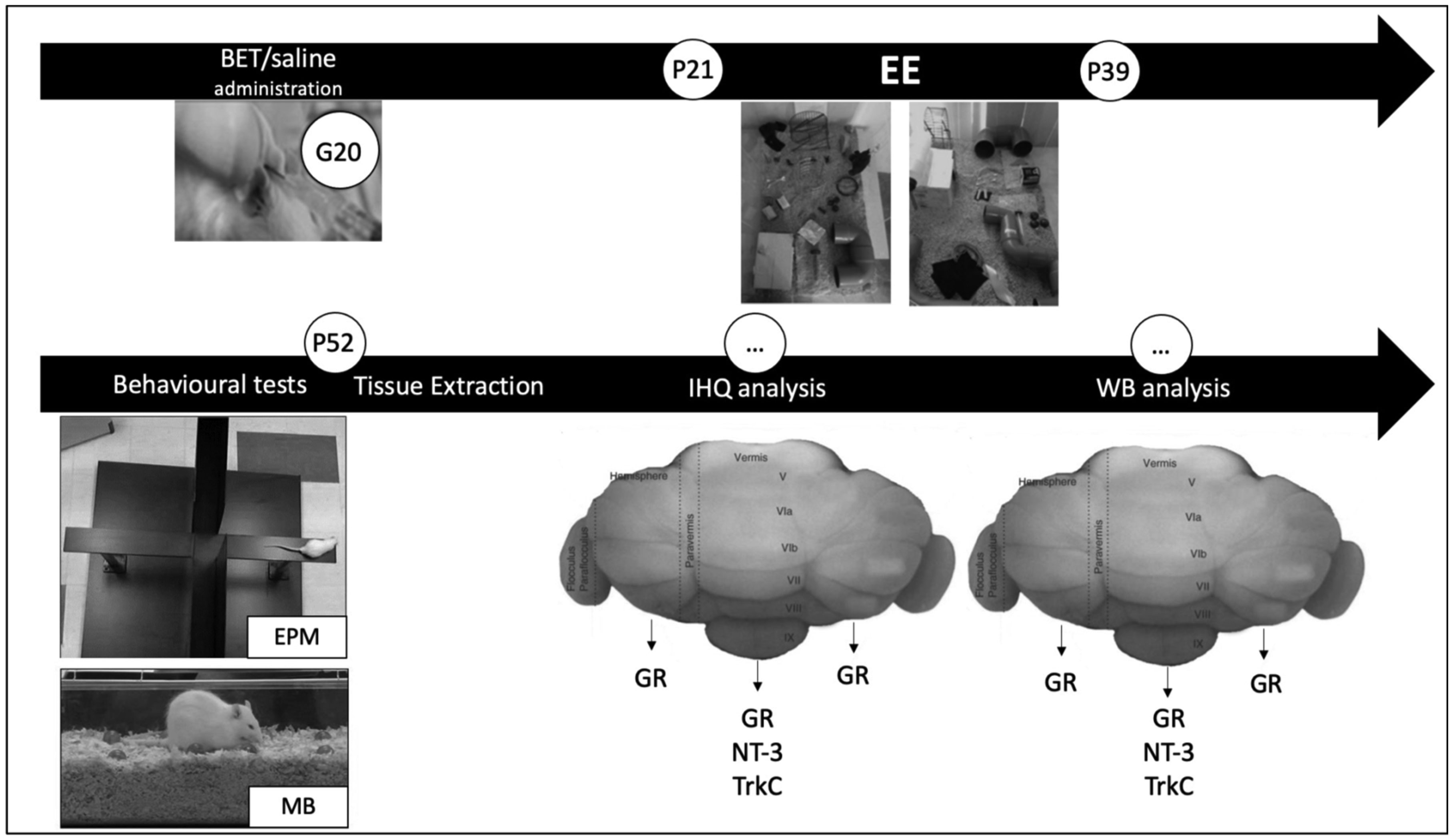
During prenatal life, exposure to synthetic glucocorticoids (SGCs) can alter normal foetal development, resulting in disease later in life. Previously, we have shown alterations in the dendritic cytoarchitecture of Purkinje cells in adolescent rat progeny prenatally exposed to glucocorticoids. However, the molecular mechanisms underlying these alterations remain unclear. A possible molecular candidate whose deregulation may underlie these changes is the glucocorticoid receptor (GR) and neurotrophin 3/ tropomyosin receptor kinase C, neurotrophic complex (NT-3/TrkC), which specifically modulates the development of the neuronal connections in the cerebellar vermis. To date, no evidence has shown that the cerebellar expression levels of this neurotrophic complex are affected by exposure to a synthetic glucocorticoid in utero. Therefore, the first objective of this investigation was to evaluate the expression of GR, NT-3 and TrkC in the cerebellar vermis using immunohistochemistry and western blot techniques by evaluating the progeny during the postnatal stage equivalent to adolescence (postnatal Day 52). Additionally, we evaluated anxiety-like behaviours in progeny using the elevated plus maze and the marble burying test. In addition, an environmental enrichment (EE) can increase the expression of some neurotrophins and has anxiolytic power. Therefore, we wanted to assess whether an EE reversed the long-term alterations induced by prenatal betamethasone exposure. The major findings of this study were as follows: i) prenatal betamethasone (BET) administration decreases GR, NT-3 and TrkC expression in the cerebellar vermis ii) prenatal BET administration decreases GR expression in the cerebellar hemispheres and iii) enhances the anxiety-like behaviours in the same progeny, and iv) exposure to an EE reverses the reduced expression of GR, NT-3 and TrkC in the cerebellar vermis and v) decreases anxiety-like behaviours. In conclusion, an enriched environment applied 18 days post-weaning was able to restabilize GR, NT-3 and TrkC expression levels and reverse anxious behaviours observed in adolescent rats prenatally exposed to betamethasone.
Citation: Martina Valencia, Odra Santander, Eloísa Torres, Natali Zamora, Fernanda Muñoz, Rodrigo Pascual. Environmental enrichment reverses cerebellar impairments caused by prenatal exposure to a synthetic glucocorticoid[J]. AIMS Neuroscience, 2022, 9(3): 320-344. doi: 10.3934/Neuroscience.2022018
During prenatal life, exposure to synthetic glucocorticoids (SGCs) can alter normal foetal development, resulting in disease later in life. Previously, we have shown alterations in the dendritic cytoarchitecture of Purkinje cells in adolescent rat progeny prenatally exposed to glucocorticoids. However, the molecular mechanisms underlying these alterations remain unclear. A possible molecular candidate whose deregulation may underlie these changes is the glucocorticoid receptor (GR) and neurotrophin 3/ tropomyosin receptor kinase C, neurotrophic complex (NT-3/TrkC), which specifically modulates the development of the neuronal connections in the cerebellar vermis. To date, no evidence has shown that the cerebellar expression levels of this neurotrophic complex are affected by exposure to a synthetic glucocorticoid in utero. Therefore, the first objective of this investigation was to evaluate the expression of GR, NT-3 and TrkC in the cerebellar vermis using immunohistochemistry and western blot techniques by evaluating the progeny during the postnatal stage equivalent to adolescence (postnatal Day 52). Additionally, we evaluated anxiety-like behaviours in progeny using the elevated plus maze and the marble burying test. In addition, an environmental enrichment (EE) can increase the expression of some neurotrophins and has anxiolytic power. Therefore, we wanted to assess whether an EE reversed the long-term alterations induced by prenatal betamethasone exposure. The major findings of this study were as follows: i) prenatal betamethasone (BET) administration decreases GR, NT-3 and TrkC expression in the cerebellar vermis ii) prenatal BET administration decreases GR expression in the cerebellar hemispheres and iii) enhances the anxiety-like behaviours in the same progeny, and iv) exposure to an EE reverses the reduced expression of GR, NT-3 and TrkC in the cerebellar vermis and v) decreases anxiety-like behaviours. In conclusion, an enriched environment applied 18 days post-weaning was able to restabilize GR, NT-3 and TrkC expression levels and reverse anxious behaviours observed in adolescent rats prenatally exposed to betamethasone.

| [1] |
Gutteling BM, de Weerth C, Zandbelt N, et al. (2006) Does maternal prenatal stress adversely affect the child's learning and memory at age six?. J Abnorm Child Psychol 34: 789-798. https://doi.org/10.1007/s10802-006-9054-7 
|
| [2] |
Cirulli F, Francia N, Berry A, et al. (2009) Early life stress as a risk factor for mental health: role of neurotrophins from rodents to non-human primates. Neurosci Biobehav Rev 33: 573-585. https://doi.org/10.1016/j.neubiorev.2008.09.001
|
| [3] |
Lunghi L, Pavan B, Biondi C, et al. (2010) Use of glucocorticoids in pregnancy. Curr Pharm Des 16: 3616-3637. https://doi.org/10.2174/138161210793797898
|
| [4] |
Alexander N, Rosenlocher F, Stalder T, et al. (2012) Impact of antenatal synthetic glucocorticoid exposure on endocrine stress reactivity in term-born children. J Clin Endocrinol Metab 97: 3538-3544. https://doi.org/10.1210/jc.2012-1970
|
| [5] |
Stalnacke J, Diaz Heijtz R, Norberg H, et al. (2013) Cognitive outcome in adolescents and young adults after repeat courses of antenatal corticosteroids. J Pediatr 163: 441-446. https://doi.org/10.1016/j.jpeds.2013.01.030
|
| [6] |
Bustamante C, Valencia M, Torres C, et al. (2014) Effects of a single course of prenatal betamethasone on dendritic development in dentate gyrus granular neurons and on spatial memory in rat offspring. Neuropediatrics 45: 354-361. https://doi.org/10.1055/s-0034-1387167
|
| [7] | Pascual R, Valencia M, Larrea S, et al. (2014) Single course of antenatal betamethasone produces delayed changes in morphology and calbindin-D28k expression in a rat's cerebellar Purkinje cells. Acta Neurobiol Exp (Wars) 74: 415-423. |
| [8] |
Peffer ME, Zhang JY, Umfrey L, et al. (2015) Minireview: the impact of antenatal therapeutic synthetic glucocorticoids on the developing fetal brain. Mol Endocrinol 29: 658-666. https://doi.org/10.1210/me.2015-1042
|
| [9] |
Pascual R, Valencia M, Bustamante C (2015a) Antenatal betamethasone produces protracted changes in anxiety-like behaviors and in the expression of microtubule-associated protein 2, brain-derived neurotrophic factor and the tyrosine kinase B receptor in the rat cerebellar cortex. Int J Dev Neurosci 43: 78-85. https://doi.org/10.1016/j.ijdevneu.2015.04.005
|
| [10] | Pascual R, Valencia M, Bustamante C (2015b) Purkinje cell dendritic atrophy induced by prenatal stress is mitigated by early environmental enrichment. Neuropediatrics 46: 37-43. https://doi.org/10.1055/s-0034-1395344 |
| [11] |
Zeng Y, Brydges NM, Wood ER, et al. (2015) Prenatal glucocorticoid exposure in rats: programming effects on stress reactivity and cognition in adult offspring. Stress 18: 353-361. https://doi.org/10.3109/10253890.2015.1055725
|
| [12] |
Pascual R, Valencia M, Bustamante C (2016) Effect of antenatal betamethasone administration on rat cerebellar expression of type la metabotropic glutamate receptors (mGluRla) and anxiety-like behavior in the elevated plus maze. Clin Exp Obstet Gynecol 43: 534-538. https://doi.org/10.12891/ceog3016.2016
|
| [13] | Sun Y, Wan X, Ouyang J, et al. (2016) Prenatal Dexamethasone Exposure Increases the Susceptibility to Autoimmunity in Offspring Rats by Epigenetic Programing of Glucocorticoid Receptor. Biomed Res Int 2016: 9409452. https://doi.org/10.1155/2016/9409452 |
| [14] |
Pascual R, Cuevas I, Santander O, et al. (2017) Influence of antenatal synthetic glucocorticoid administration on pyramidal cell morphology and microtubule-associated protein type 2 (MAP2) in rat cerebrocortical neurons. Clin Pediatr Endocrinol 26: 9-15. https://doi.org/10.1297/cpe.26.9
|
| [15] |
Marciniak B, Patro-Małysza J, Poniedziałek-Czajkowska E, et al. (2011) Glucocorticoids in pregnancy. Curr Pharma Biotechno 12: 750-757. https://doi.org/10.2174/138920111795470868
|
| [16] |
Davis EP, Sandman CA, Buss C, et al. (2013) Fetal glucocorticoid exposure is associated with preadolescent brain development. Biol Psychiatry 74: 647-655. https://doi.org/10.1016/j.biopsych.2013.03.009
|
| [17] |
Skorzewska A, Lehner M, Wislowska-Stanek A, et al. (2014) The effect of chronic administration of corticosterone on anxiety- and depression-like behavior and the expression of GABA-A receptor alpha-2 subunits in brain structures of low- and high-anxiety rats. Horm Behav 65: 6-13. https://doi.org/10.1016/j.yhbeh.2013.10.011
|
| [18] |
Erni K, Shaqiri-Emini L, La Marca R, et al. (2012) Psychobiological effects of prenatal glucocorticoid exposure in 10-year-old-children. Front Psychiatry 3: 104. https://doi.org/10.3389/fpsyt.2012.00104
|
| [19] |
Winston JH, Li Q, Sarna SK (2014) Chronic prenatal stress epigenetically modifies spinal cord BDNF expression to induce sex-specific visceral hypersensitivity in offspring. Neurogastroenterol Motil 26: 715-730. https://doi.org/10.1111/nmo.12326
|
| [20] |
Perroud N, Rutembesa E, Paoloni-Giacobino A, et al. (2014) The Tutsi genocide and transgenerational transmission of maternal stress: epigenetics and biology of the HPA axis. World J Biol Psychiatry 15: 334-345. https://doi.org/10.3109/15622975.2013.866693
|
| [21] |
Hiroi R, Carbone DL, Zuloaga DG, et al. (2016) Sex-dependent programming effects of prenatal glucocorticoid treatment on the developing serotonin system and stress-related behaviors in adulthood. Neuroscience 320: 43-56. https://doi.org/10.1016/j.neuroscience.2016.01.055
|
| [22] |
Tsiarli MA, Rudine A, Kendall N, et al. (2017) Antenatal dexamethasone exposure differentially affects distinct cortical neural progenitor cells and triggers long-term changes in murine cerebral architecture and behavior. Transl Psychiatry 7: e1153. https://doi.org/10.1038/tp.2017.65
|
| [23] |
Liu PZ, Nusslock R (2018) How Stress Gets Under the Skin: Early Life Adversity and Glucocorticoid Receptor Epigenetic Regulation. Curr Genomics 19: 653-664. https://doi.org/10.2174/1389202919666171228164350
|
| [24] |
Noorlander CW, Visser GH, Ramakers GM, et al. (2008) Prenatal corticosteroid exposure affects hippocampal plasticity and reduces lifespan. Dev Neurobiol 68: 237-246. https://doi.org/10.1002/dneu.20583
|
| [25] |
Hauser J, Feldon J, Pryce CR (2009) Direct and dam-mediated effects of prenatal dexamethasone on emotionality, cognition and HPA axis in adult Wistar rats. Horm Behav 56: 364-375. https://doi.org/10.1016/j.yhbeh.2009.07.003
|
| [26] |
Gjerstad JK, Lightman SL, Spiga F (2018) Role of glucocorticoid negative feedback in the regulation of HPA axis pulsatility. Stress 21: 403-416. https://doi.org/10.1080/10253890.2018.1470238
|
| [27] |
Meijer OC, Koorneef LL, Kroon J (2018) Glucocorticoid receptor modulators. Ann Endocrinol (Paris) 79: 107-111. https://doi.org/10.1016/j.ando.2018.03.004
|
| [28] |
Harle G, Lalonde R, Fonte C, et al. (2017) Repeated corticosterone injections in adult mice alter stress hormonal receptor expression in the cerebellum and motor coordination without affecting spatial learning. Behav Brain Res 326: 121-131. https://doi.org/10.1016/j.bbr.2017.02.035
|
| [29] |
Noguchi KK, Lau K, Smith DJ, et al. (2011) Glucocorticoid receptor stimulation and the regulation of neonatal cerebellar neural progenitor cell apoptosis. Neurobiol Dis 43: 356-363. https://doi.org/10.1016/j.nbd.2011.04.004
|
| [30] |
Carta I, Chen CH, Schott AL, et al. (2019) Cerebellar modulation of the reward circuitry and social behavior. Science 363: eaav0581. https://doi.org/10.1126/science.aav0581
|
| [31] |
Stoodley CJ, D'Mello AM, Ellegood J, et al. (2017) Altered cerebellar connectivity in autism and cerebellar-mediated rescue of autism-related behaviors in mice. Nat Neurosci 20: 1744-1751. https://doi.org/10.1038/s41593-017-0004-1
|
| [32] |
Schmahmann JD, Caplan D (2006) Cognition emotion and the cerebellum. Brain 129: 290-292. https://doi.org/10.1093/brain/awh729
|
| [33] |
Schutter DJ (2012) The cerebello-hypothalamic-pituitary-adrenal axis dysregulation hypothesis in depressive disorder. Med Hypotheses 79: 779-783. https://doi.org/10.1016/j.mehy.2012.08.027
|
| [34] |
Ulupinar E, Yucel F (2005) Prenatal stress reduces interneuronal connectivity in the rat cerebellar granular layer. Neurotoxicol Teratol 27: 475-484. https://doi.org/10.1016/j.ntt.2005.01.015
|
| [35] |
Holm SK, Madsen KS, Vestergaard M, et al. (2018) Total brain, cortical, and white matter volumes in children previously treated with glucocorticoids. Pediatr Res 83: 804-812. https://doi.org/10.1038/pr.2017.312
|
| [36] |
Valencia M, Illanes J, Santander O, et al. (2019) Environmental enrichment restores the reduced expression of cerebellar synaptophysin and the motor coordination impairment in rats prenatally treated with betamethasone. Physiol Behav 209: 112590. https://doi.org/10.1016/j.physbeh.2019.112590
|
| [37] |
Lindholm D, Castren E, Tsoulfas P, et al. (1993) Neurotrophin-3 induced by tri-iodothyronine in cerebellar granule cells promotes Purkinje cell differentiation. J Cell Biol 122: 443-450. https://doi.org/10.1083/jcb.122.2.443
|
| [38] |
Mount HT, Dreyfus CF, Black IB (1994) Neurotrophin-3 selectively increases cultured Purkinje cell survival. Neuroreport 5: 2497-2500. https://doi.org/10.1097/00001756-199412000-00023
|
| [39] |
Minichiello L, Klein R (1996) TrkB and TrkC neurotrophin receptors cooperate in promoting survival of hippocampal and cerebellar granule neurons. Genes Dev 10: 2849-2858. https://doi.org/10.1101/gad.10.22.2849
|
| [40] |
Velier JJ, Ellison JA, Fisher RS, et al. (1997) The trkC receptor is transiently localized to Purkinje cell dendrites during outgrowth and maturation in the rat. J Neurosci Res 50: 649-656. https://doi.org/10.1002/(SICI)1097-4547(19971115)50:4<649::AID-JNR15>3.0.CO;2-Y
|
| [41] |
Bates B, Rios M, Trumpp A, et al. (1999) Neurotrophin-3 is required for proper cerebellar development. Nat Neurosci 2: 115-117. https://doi.org/10.1038/5669
|
| [42] |
Ramos B, Valin A, Sun X, et al. (2009) Sp4-dependent repression of neurotrophin-3 limits dendritic branching. Mol Cell Neurosci 42: 152-159. https://doi.org/10.1016/j.mcn.2009.06.008
|
| [43] |
Joo W, Hippenmeyer S, Luo L (2014) Neurodevelopment. Dendrite morphogenesis depends on relative levels of NT-3/TrkC signaling. Science 346: 626-629. https://doi.org/10.1126/science.1258996
|
| [44] |
Han KA, Woo D, Kim S, et al. (2016) Neurotrophin-3 Regulates Synapse Development by Modulating TrkC-PTPsigma Synaptic Adhesion and Intracellular Signaling Pathways. J Neurosci 36: 4816-4831. https://doi.org/10.1523/JNEUROSCI.4024-15.2016
|
| [45] |
Dedoni S, Olianas MC, Ingianni A, et al. (2017) Interferon-beta Inhibits Neurotrophin 3 Signalling and Pro-Survival Activity by Upregulating the Expression of Truncated TrkC-T1 Receptor. Mol Neurobiol 54: 1825-1843. https://doi.org/10.1007/s12035-016-9789-2
|
| [46] |
Ramos-Languren LE, Escobar ML (2013) Plasticity and metaplasticity of adult rat hippocampal mossy fibers induced by neurotrophin-3. Eur J Neurosci 37: 1248-1259. https://doi.org/10.1111/ejn.12141
|
| [47] |
Ammendrup-Johnsen I, Naito Y, Craig AM, et al. (2015) Neurotrophin-3 Enhances the Synaptic Organizing Function of TrkC-Protein Tyrosine Phosphatase sigma in Rat Hippocampal Neurons. J Neurosci 35: 12425-12431. https://doi.org/10.1523/JNEUROSCI.1330-15.2015
|
| [48] |
Neveu I, Arenas E (1996) Neurotrophins promote the survival and development of neurons in the cerebellum of hypothyroid rats in vivo. J Cell Biol 133: 631-646. https://doi.org/10.1083/jcb.133.3.631
|
| [49] |
McCreary JK, Erickson ZT, Hao Y, et al. (2016) Environmental Intervention as a Therapy for Adverse Programming by Ancestral Stress. Sci Rep 6: 37814. https://doi.org/10.1038/srep37814
|
| [50] |
McCreary JK, Metz G (2016) Environmental enrichment as an intervention for adverse health outcomes of prenatal stress. Environ Epigenet 2: dvw013. https://doi.org/10.1093/eep/dvw013
|
| [51] |
McQuaid RJ, Dunn R, Jacobson-Pick S, et al. (2018) Post-weaning Environmental Enrichment in Male CD-1 Mice: Impact on Social Behaviors, Corticosterone Levels and Prefrontal Cytokine Expression in Adulthood. Front Behav Neurosci 12: 145. https://doi.org/10.3389/fnbeh.2018.00145
|
| [52] |
Murueta-Goyena A, Ortuzar N, Gargiulo PA, et al. (2018) Short-Term Exposure to Enriched Environment in Adult Rats Restores MK-801-Induced Cognitive Deficits and GABAergic Interneuron Immunoreactivity Loss. Mol Neurobiol 55: 26-41. https://doi.org/10.1007/s12035-017-0715-z
|
| [53] |
Sparling JE, Baker SL, Bielajew C (2018) Effects of combined pre- and post-natal enrichment on anxiety-like, social, and cognitive behaviours in juvenile and adult rat offspring. Behav Brain Res 353: 40-50. https://doi.org/10.1016/j.bbr.2018.06.033
|
| [54] |
Vazquez-Sanroman D, Sanchis-Segura C, Toledo R, et al. (2013) The effects of enriched environment on BDNF expression in the mouse cerebellum depending on the length of exposure. Behav Brain Res 243: 118-128. https://doi.org/10.1016/j.bbr.2012.12.047
|
| [55] |
Hu YS, Long N, Pigino G, et al. (2013) Molecular mechanisms of environmental enrichment: impairments in Akt/GSK3beta, neurotrophin-3 and CREB signaling. PLoS One 8: e64460. https://doi.org/10.1371/journal.pone.0064460
|
| [56] |
Rogers J, Li S, Lanfumey L, et al. (2017) Environmental enrichment reduces innate anxiety with no effect on depression-like behaviour in mice lacking the serotonin transporter. Behav Brain Res 332: 355-361. https://doi.org/10.1016/j.bbr.2017.06.009
|
| [57] |
Ashokan A, Hegde A, Balasingham A, et al. (2018) Housing environment influences stress-related hippocampal substrates and depression-like behavior. Brain Res 1683: 78-85. https://doi.org/10.1016/j.brainres.2018.01.021
|
| [58] |
Angelucci F, De Bartolo P, Gelfo F, et al. (2009) Increased concentrations of nerve growth factor and brain-derived neurotrophic factor in the rat cerebellum after exposure to environmental enrichment. Cerebellum 8: 499-506. https://doi.org/10.1007/s12311-009-0129-1
|
| [59] |
Paban V, Chambon C, Manrique C, et al. (2011) Neurotrophic signaling molecules associated with cholinergic damage in young and aged rats: environmental enrichment as potential therapeutic agent. Neurobiol Aging 32: 470-485. https://doi.org/10.1016/j.neurobiolaging.2009.03.010
|
| [60] |
Jain V, Baitharu I, Prasad D, et al. (2013) Enriched environment prevents hypobaric hypoxia induced memory impairment and neurodegeneration: role of BDNF/PI3K/GSK3beta pathway coupled with CREB activation. PLoS One 8: e62235. https://doi.org/10.1371/journal.pone.0062235
|
| [61] |
Bahi A (2017) Environmental enrichment reduces chronic psychosocial stress-induced anxiety and ethanol-related behaviors in mice. Prog Neuropsychopharmacol Biol Psychiatry 77: 65-74. https://doi.org/10.1016/j.pnpbp.2017.04.001
|
| [62] | Slater AM, Cao L (2015) A protocol for housing mice in an enriched environment. J Vis Exp : e52874. https://doi.org/10.3791/52874 |
| [63] |
Cintoli S, Cenni MC, Pinto B, et al. (2018) Environmental Enrichment Induces Changes in Long-Term Memory for Social Transmission of Food Preference in Aged Mice through a Mechanism Associated with Epigenetic Processes. Neural Plast 2018: 3725087. https://doi.org/10.1155/2018/3725087
|
| [64] |
Kedia S, Chattarji S (2014) Marble burying as a test of the delayed anxiogenic effects of acute immobilisation stress in mice. J Neurosci Methods 233: 150-154. https://doi.org/10.1016/j.jneumeth.2014.06.012
|
| [65] |
de Brouwer G, Wolmarans W (2018) Back to basics: A methodological perspective on marble-burying behavior as a screening test for psychiatric illness. Behav Proc 157: 590-600. https://doi.org/10.1016/j.beproc.2018.04.011
|
| [66] | Paxinos G, Watson C (2007) The rat brain, in stereotaxic coordinates. San Diego: Academic Press. |
| [67] |
Lakens D (2013) Calculating and reporting effect sizes to facilitate cumulative science: a practical primer for t-tests and ANOVAs. Front Psychol 4: 863. https://doi.org/10.3389/fpsyg.2013.00863
|
| [68] |
McGowan PO, Sasaki A, D'Alessio AC, et al. (2009) Epigenetic regulation of the glucocorticoid receptor in human brain associates with childhood abuse. Nat Neurosci 12: 342-348. https://doi.org/10.1038/nn.2270
|
| [69] |
Moisiadis VG, Matthews SG (2014) Glucocorticoids and fetal programming part 1: Outcomes. Nat Rev Endocrinol 10: 391-402. https://doi.org/10.1038/nrendo.2014.73
|
| [70] |
Conradt E, Lester BM, Appleton AA, et al. (2013) The roles of DNA methylation of NR3C1 and 11beta-HSD2 and exposure to maternal mood disorder in utero on newborn neurobehavior. Epigenetics 8: 1321-1329. https://doi.org/10.4161/epi.26634
|
| [71] |
van der Knaap LJ, Riese H, Hudziak JJ, et al. (2014) Glucocorticoid receptor gene (NR3C1) methylation following stressful events between birth and adolescence. The TRAILS study. Transl Psychiatry 4: e381. https://doi.org/10.1038/tp.2014.22
|
| [72] |
Murgatroyd C, Quinn JP, Sharp HM, et al. (2015) Effects of prenatal and postnatal depression, and maternal stroking, at the glucocorticoid receptor gene. Transl Psychiatry 5: e560. https://doi.org/10.1038/tp.2014.140
|
| [73] |
Arabska J, Lucka A, Strzelecki D, et al. (2018) In schizophrenia serum level of neurotrophin-3 (NT-3) is increased only if depressive symptoms are present. Neurosci Lett 684: 152-155. https://doi.org/10.1016/j.neulet.2018.08.005
|
| [74] |
Wagner MJ, Kim TH, Savall J, et al. (2017) Cerebellar granule cells encode the expectation of reward. Nature 544: 96-100. https://doi.org/10.1038/nature21726
|
| [75] |
Ashokan A, Hegde A, Mitra R (2016) Short-term environmental enrichment is sufficient to counter stress-induced anxiety and associated structural and molecular plasticity in basolateral amygdala. Psychoneuroendocrinology 69: 189-196. https://doi.org/10.1016/j.psyneuen.2016.04.009
|
| [76] |
Novaes LS, Dos Santos NB, Batalhote RFP, et al. (2017) Environmental enrichment protects against stress-induced anxiety: Role of glucocorticoid receptor, ERK, and CREB signaling in the basolateral amygdala. Neuropharmacology 113: 457-466. https://doi.org/10.1016/j.neuropharm.2016.10.026
|
| [77] |
Leger M, Paizanis E, Dzahini K, et al. (2015) Environmental Enrichment Duration Differentially Affects Behavior and Neuroplasticity in Adult Mice. Cereb Cortex : 4048-4061. https://doi.org/10.1093/cercor/bhu119
|
| [78] |
Eshra A, Hirrlinger P, Hallermann S (2019) Enriched Environment Shortens the Duration of Action Potentials in Cerebellar Granule Cells. Front Cell Neusci 13: 289. https://doi.org/10.3389/fncel.2019.00289
|


Figures(10)

Martina Valencia, Odra Santander, Eloísa Torres, Natali Zamora, Fernanda Muñoz, Rodrigo Pascual. Environmental enrichment reverses cerebellar impairments caused by prenatal exposure to a synthetic glucocorticoid[J]. AIMS Neuroscience, 2022, 9(3): 320-344. doi: 10.3934/Neuroscience.2022018


 DownLoad: