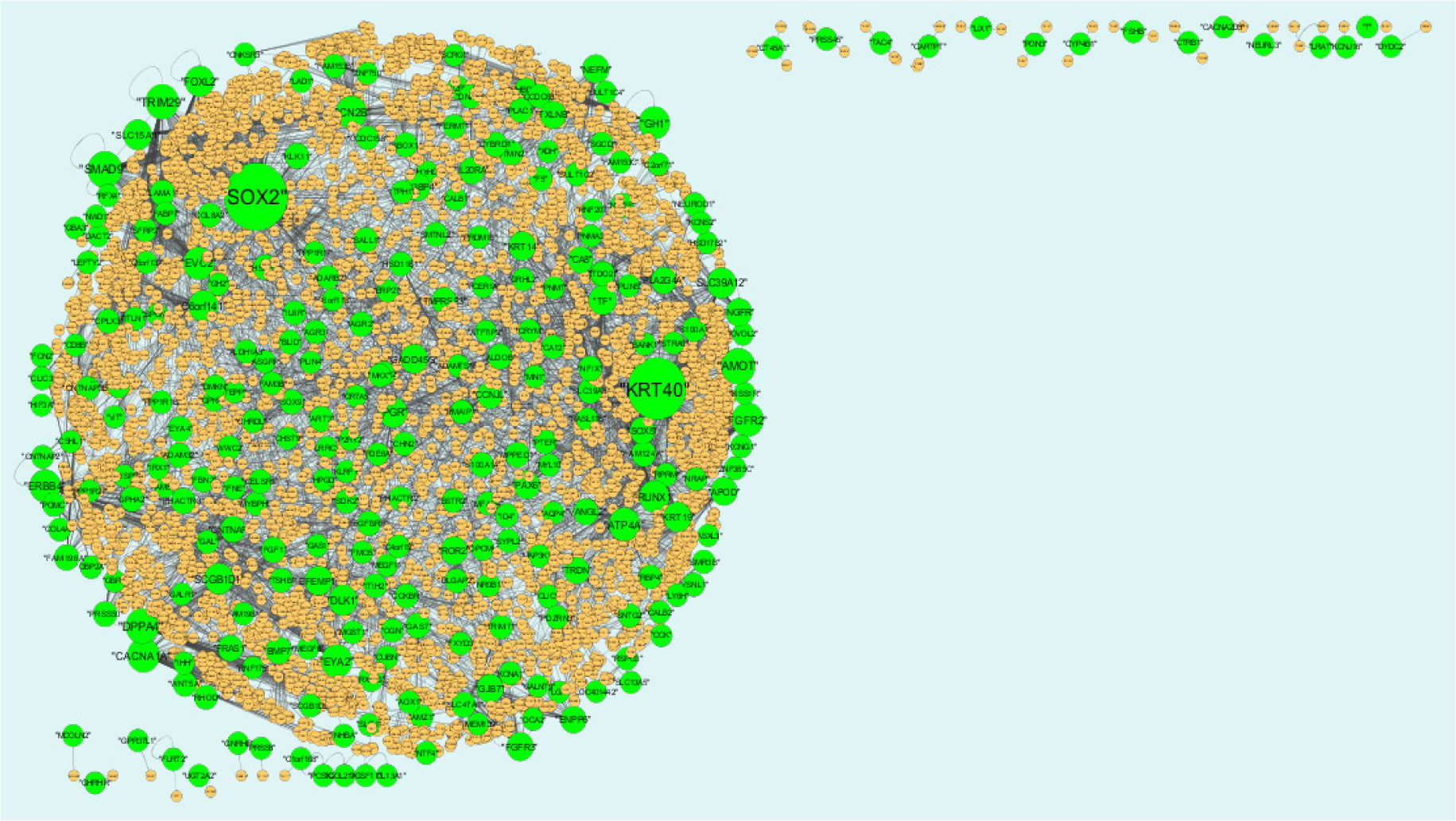
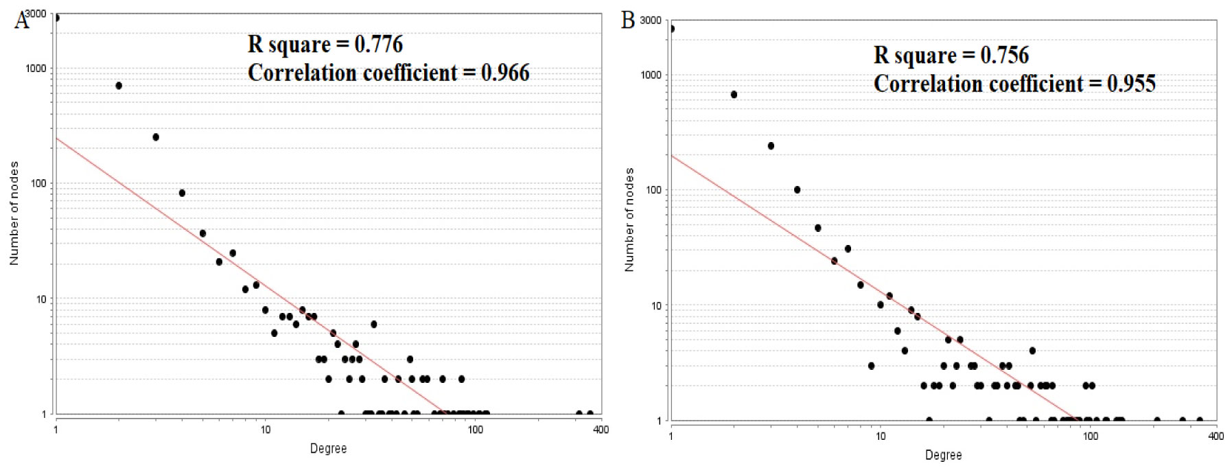
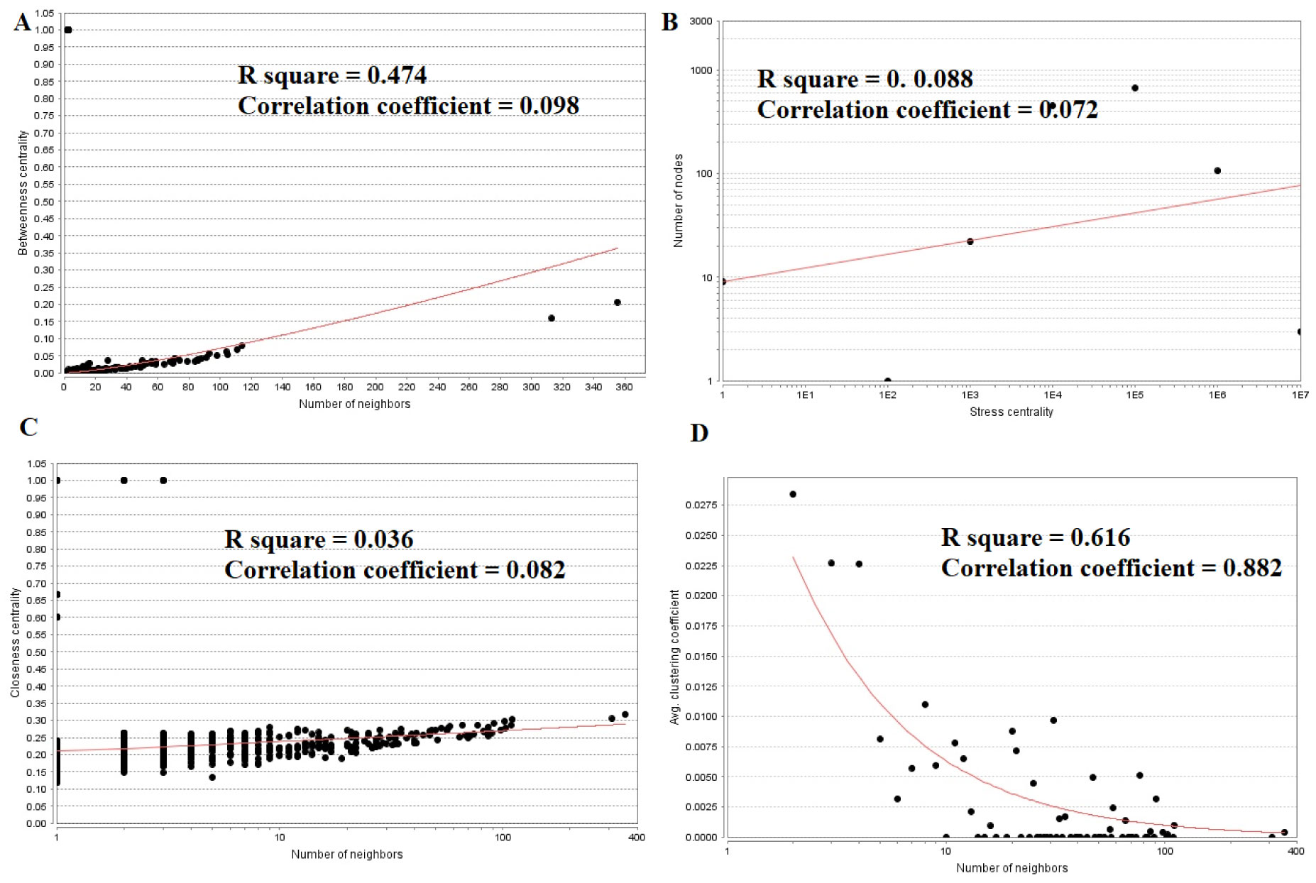
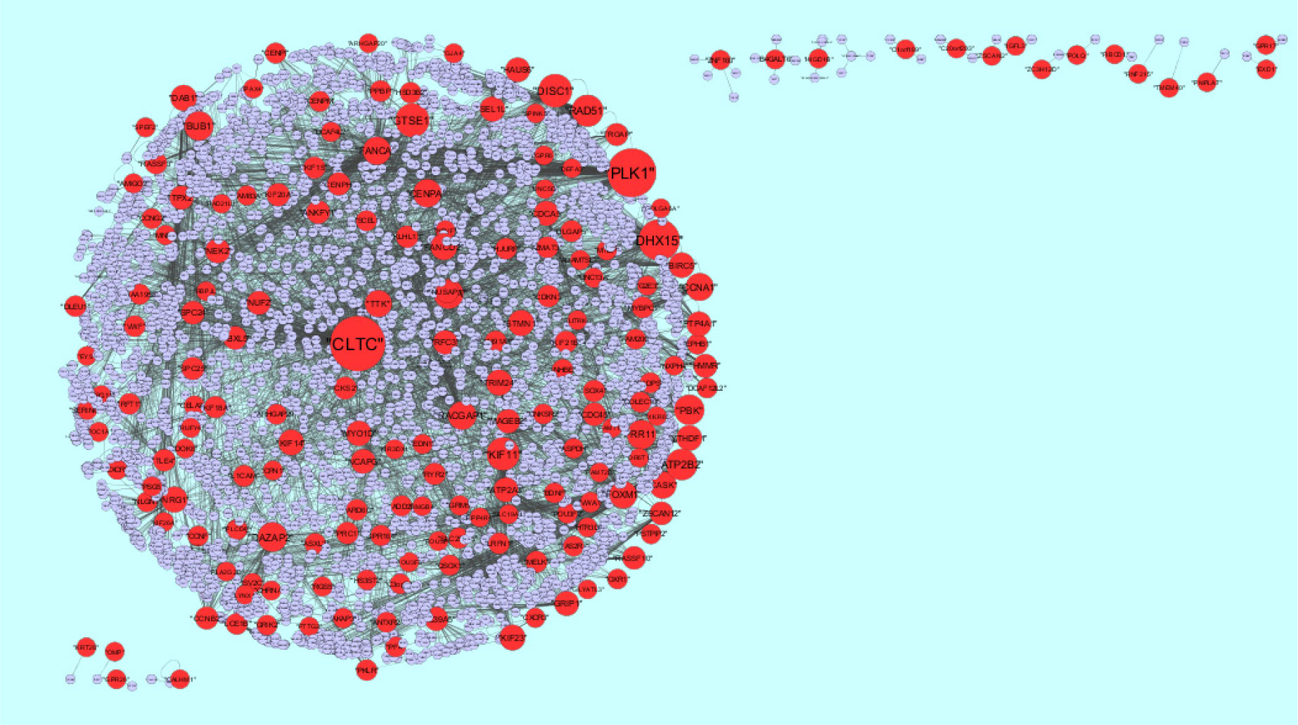
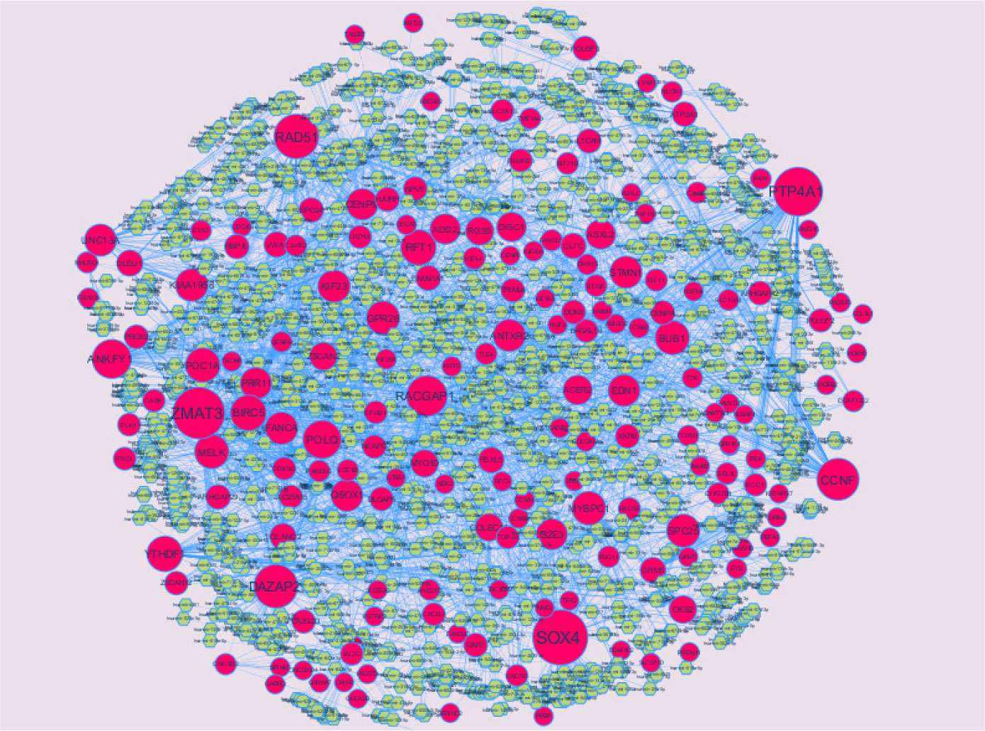
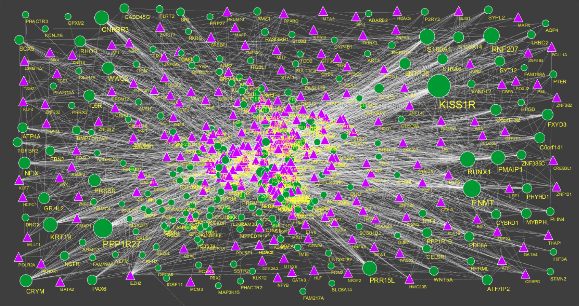
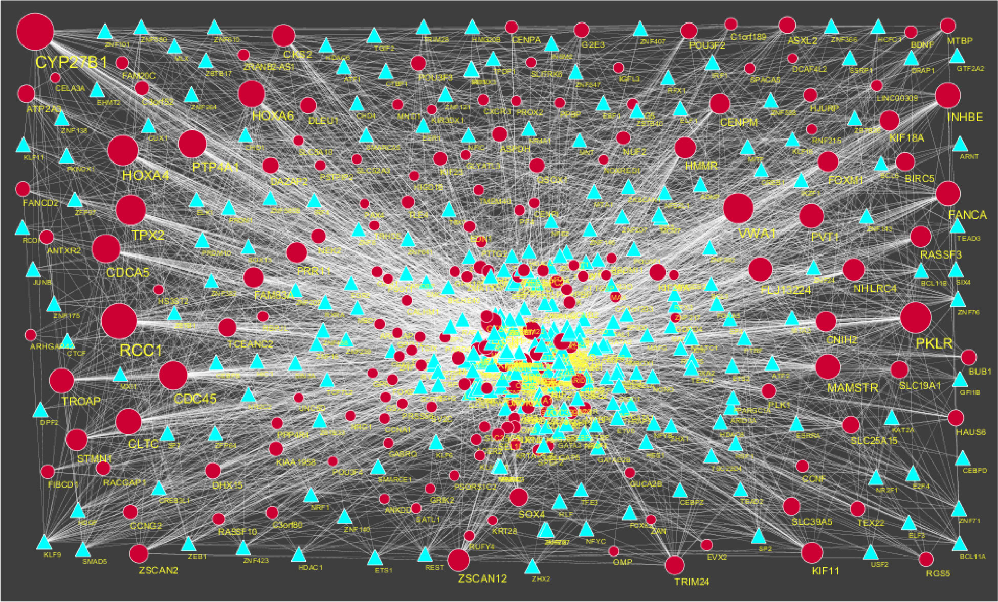
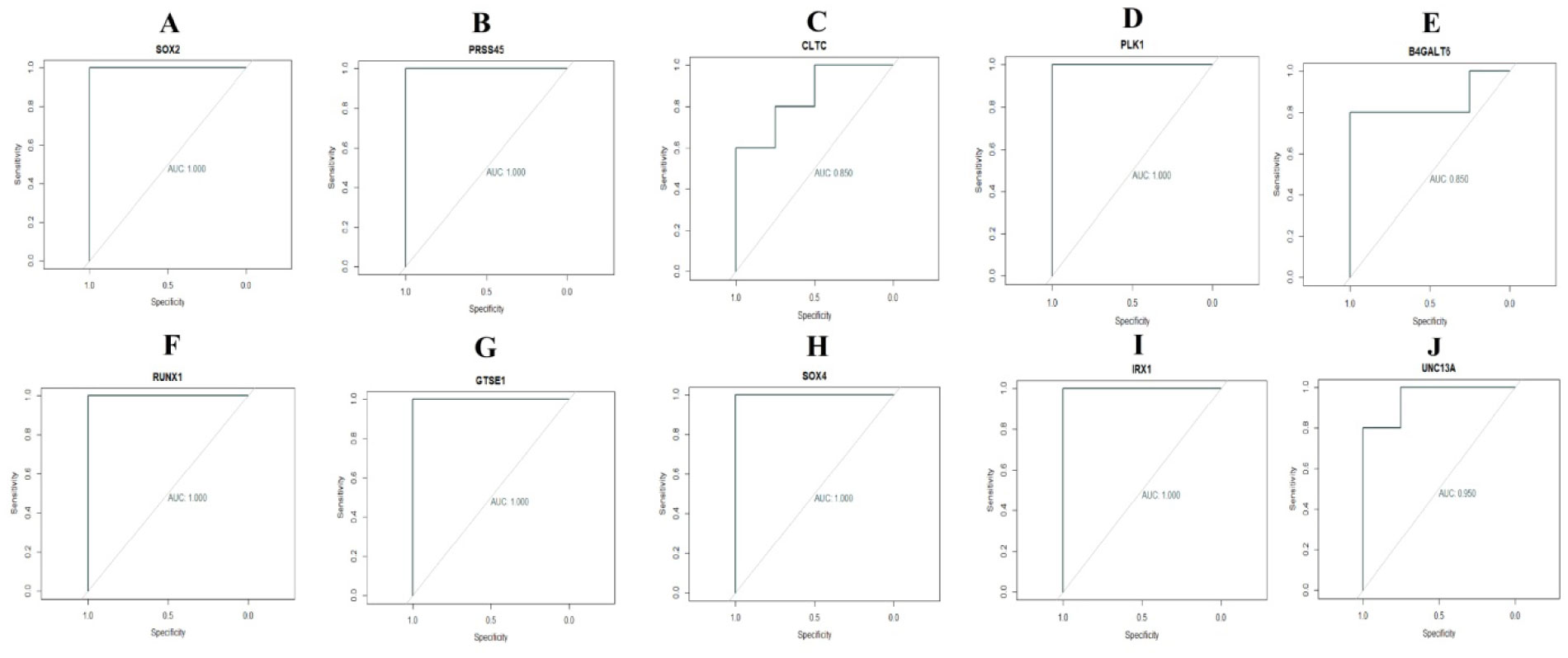
Pituitary prolactinoma is one of the most complicated and fatally pathogenic pituitary adenomas. Therefore, there is an urgent need to improve our understanding of the underlying molecular mechanism that drives the initiation, progression, and metastasis of pituitary prolactinoma. The aim of the present study was to identify the key genes and signaling pathways associated with pituitary prolactinoma using bioinformatics analysis. Transcriptome microarray dataset GSE119063 was downloaded from Gene Expression Omnibus (GEO) database. Limma package in R software was used to screen DEGs. Pathway and Gene ontology (GO) enrichment analysis were conducted to identify the biological role of DEGs. A protein-protein interaction (PPI) network was constructed and analyzed by using HIPPIE database and Cytoscape software. Module analyses was performed. In addition, a target gene-miRNA regulatory network and target gene-TF regulatory network were constructed by using NetworkAnalyst and Cytoscape software. Finally, validation of hub genes by receiver operating characteristic (ROC) curve analysis. A total of 989 DEGs were identified, including 461 up regulated genes and 528 down regulated genes. Pathway enrichment analysis showed that the DEGs were significantly enriched in the retinoate biosynthesis II, signaling pathways regulating pluripotency of stem cells, ALK2 signaling events, vitamin D3 biosynthesis, cell cycle and aurora B signaling. Gene Ontology (GO) enrichment analysis showed that the DEGs were significantly enriched in the sensory organ morphogenesis, extracellular matrix, hormone activity, nuclear division, condensed chromosome and microtubule binding. In the PPI network and modules, SOX2, PRSS45, CLTC, PLK1, B4GALT6, RUNX1 and GTSE1 were considered as hub genes. In the target gene-miRNA regulatory network and target gene-TF regulatory network, LINC00598, SOX4, IRX1 and UNC13A were considered as hub genes. Using integrated bioinformatics analysis, we identified candidate genes in pituitary prolactinoma, which might improve our understanding of the molecular mechanisms of pituitary prolactinoma.
Citation: Vikrant Ghatnatti, Basavaraj Vastrad, Swetha Patil, Chanabasayya Vastrad, Iranna Kotturshetti. Identification of potential and novel target genes in pituitary prolactinoma by bioinformatics analysis[J]. AIMS Neuroscience, 2021, 8(2): 254-283. doi: 10.3934/Neuroscience.2021014
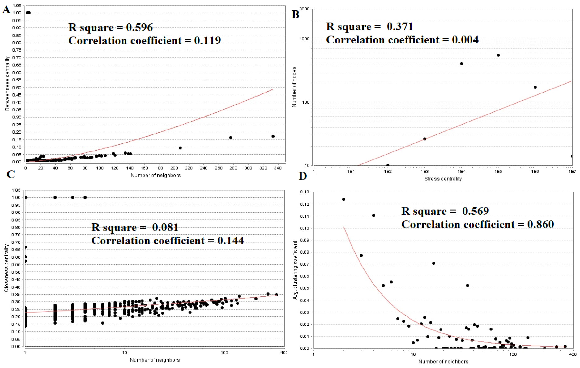
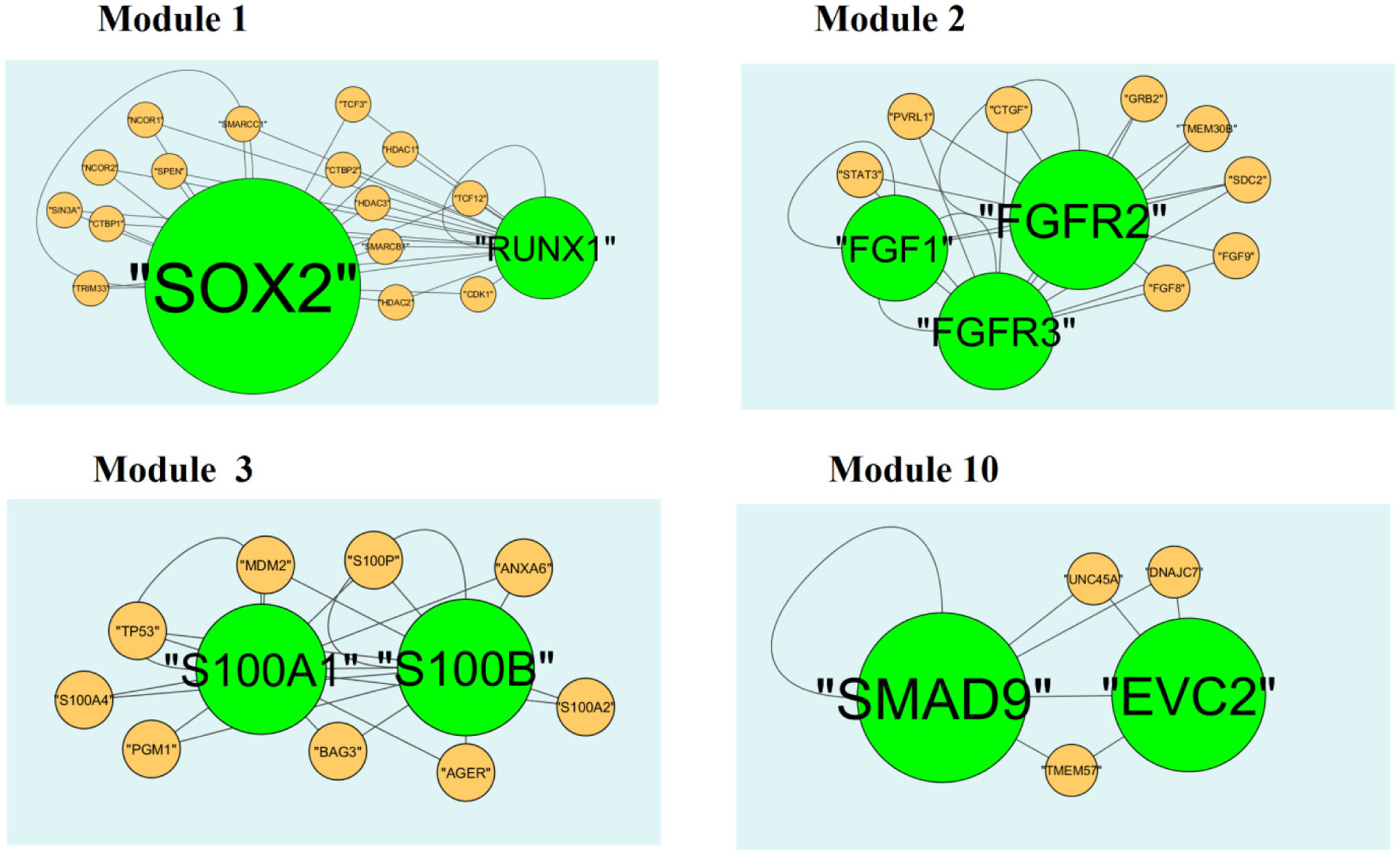
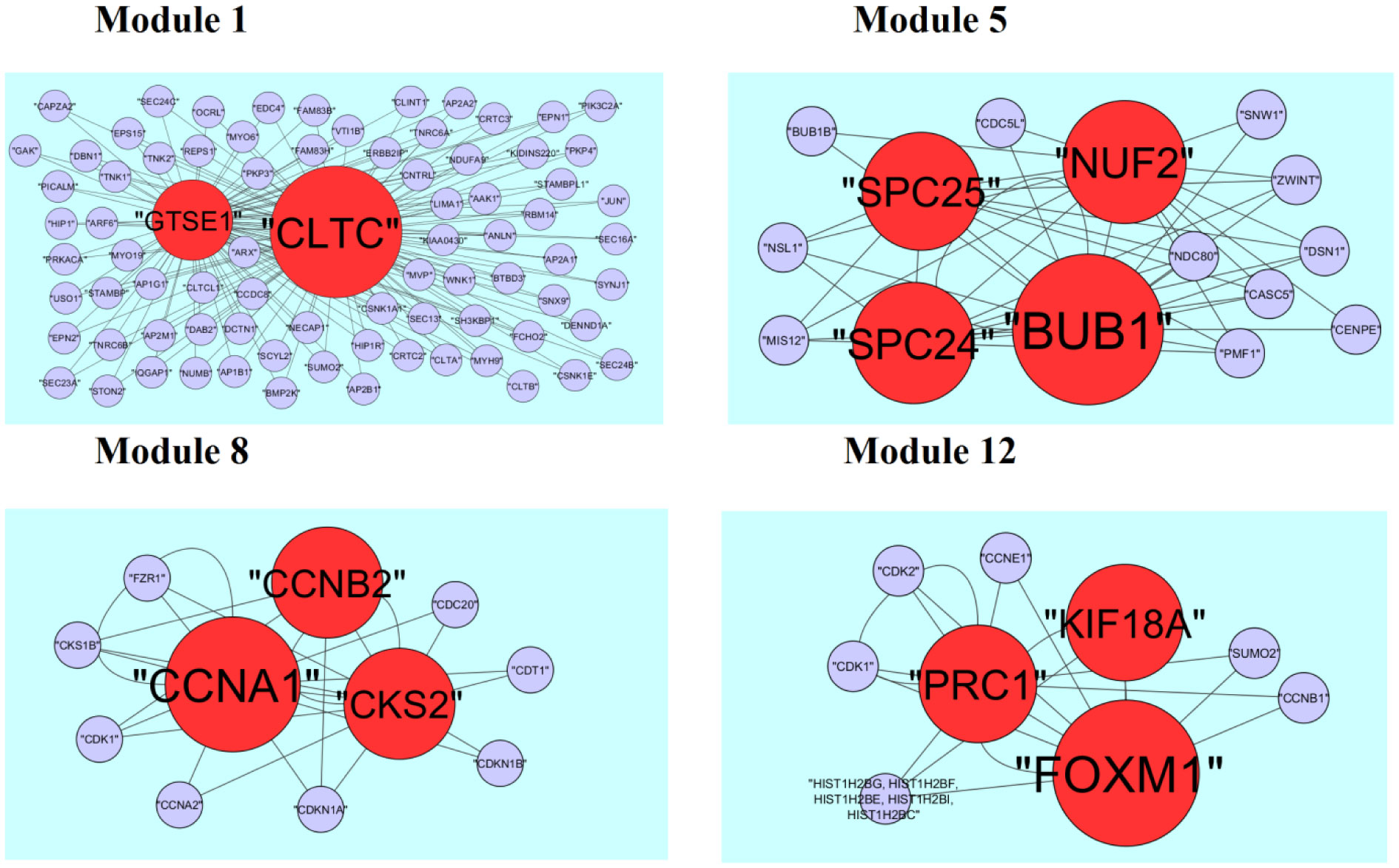
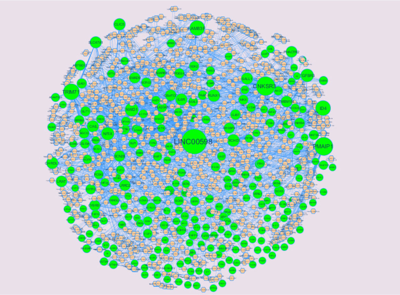
Pituitary prolactinoma is one of the most complicated and fatally pathogenic pituitary adenomas. Therefore, there is an urgent need to improve our understanding of the underlying molecular mechanism that drives the initiation, progression, and metastasis of pituitary prolactinoma. The aim of the present study was to identify the key genes and signaling pathways associated with pituitary prolactinoma using bioinformatics analysis. Transcriptome microarray dataset GSE119063 was downloaded from Gene Expression Omnibus (GEO) database. Limma package in R software was used to screen DEGs. Pathway and Gene ontology (GO) enrichment analysis were conducted to identify the biological role of DEGs. A protein-protein interaction (PPI) network was constructed and analyzed by using HIPPIE database and Cytoscape software. Module analyses was performed. In addition, a target gene-miRNA regulatory network and target gene-TF regulatory network were constructed by using NetworkAnalyst and Cytoscape software. Finally, validation of hub genes by receiver operating characteristic (ROC) curve analysis. A total of 989 DEGs were identified, including 461 up regulated genes and 528 down regulated genes. Pathway enrichment analysis showed that the DEGs were significantly enriched in the retinoate biosynthesis II, signaling pathways regulating pluripotency of stem cells, ALK2 signaling events, vitamin D3 biosynthesis, cell cycle and aurora B signaling. Gene Ontology (GO) enrichment analysis showed that the DEGs were significantly enriched in the sensory organ morphogenesis, extracellular matrix, hormone activity, nuclear division, condensed chromosome and microtubule binding. In the PPI network and modules, SOX2, PRSS45, CLTC, PLK1, B4GALT6, RUNX1 and GTSE1 were considered as hub genes. In the target gene-miRNA regulatory network and target gene-TF regulatory network, LINC00598, SOX4, IRX1 and UNC13A were considered as hub genes. Using integrated bioinformatics analysis, we identified candidate genes in pituitary prolactinoma, which might improve our understanding of the molecular mechanisms of pituitary prolactinoma.
Biological General Repository for Interaction Datasets
biological process
cellular component
Differentially Expressed Genes
Gene Expression Omnibus
Gene ontology
Human Integrated Protein-Protein Interaction rEference
Kyoto Encyclopedia of Genes and Genomes
molecular function
Small Molecule Pathway Database

| [1] |
Thorner MO, Martin WH, Rogol AD, et al. (1980) Rapid regression of pituitary prolactinomas during bromocriptine treatment. J Clin Endocrinol Metab 51: 438-445. doi: 10.1210/jcem-51-3-438

|
| [2] |
Doumith R, Gennes JL, Cabane JP, et al. (1982) Pituitary prolactinoma, adrenal aldosterone-producing adenomas, gastric schwannoma and colonic polyadenomas: a possible variant of multiple endocrine neoplasia (MEN) type I. Acta Endocrinol (Copenh) 100: 189-195. doi: 10.1530/acta.0.1000189
|
| [3] |
Oruçkaptan HH, Senmevsim O, Ozcan OE, et al. (2000) Pituitary adenomas: results of 684 surgically treated patients and review of the literature. Surg Neurol 53: 211-219. doi: 10.1016/S0090-3019(00)00171-3
|
| [4] |
Cho DY, Liau WR (2002) Comparison of endonasal endoscopic surgery and sublabial microsurgery for prolactinomas. Surg Neurol 58: 371-375. doi: 10.1016/S0090-3019(02)00892-3
|
| [5] |
Murakami M, Mizutani A, Asano S, et al. (2011) A mechanism of acquiring temozolomide resistance during transformation of atypical prolactinoma into prolactin-producing pituitary carcinoma: case report. Neurosurgery 68: E1761-E1767. doi: 10.1227/NEU.0b013e318217161a
|
| [6] |
Tsang RW, Laperriere NJ, Simpson WJ, et al. (1993) Glioma arising after radiation therapy for pituitary adenoma. A report of four patients and estimation of risk. Cancer 72: 2227-2233. doi: 10.1002/1097-0142(19931001)72:7<2227::AID-CNCR2820720727>3.0.CO;2-I
|
| [7] | Friedman E, Adams EF, Höög A, et al. (1994) Normal structural dopamine type 2 receptor gene in prolactin-secreting and other pituitary tumors. J Clin Endocrinol Metab 78: 568-574. |
| [8] |
Fedele M, Pentimalli F, Baldassarre G, et al. (2005) Transgenic mice overexpressing the wild-type form of the HMGA1 gene develop mixed growth hormone/prolactin cell pituitary adenomas and natural killer cell lymphomas. Oncogene 24: 3427-3435. doi: 10.1038/sj.onc.1208501
|
| [9] | Finelli P, Pierantoni GM, Giardino D, et al. (2002) The High Mobility Group A2 gene is amplified and overexpressed in human prolactinomas. Cancer Res 62: 2398-2405. |
| [10] |
Paez-Pereda M, Giacomini D, Refojo D, et al. (2003) Involvement of bone morphogenetic protein 4 (BMP-4) in pituitary prolactinoma pathogenesis through a Smad/estrogen receptor crosstalk. Proc Natl Acad Sci USA 100: 1034-1039. doi: 10.1073/pnas.0237312100
|
| [11] |
Shimon I, Hinton DR, Weiss MH, et al. (1998) Prolactinomas express human heparin-binding secretory transforming gene (hst) protein product: marker of tumour invasiveness. Clin Endocrinol (Oxf) 48: 23-29. doi: 10.1046/j.1365-2265.1998.00332.x
|
| [12] |
Lania AG, Ferrero S, Pivonello R, et al. (2010) Evolution of an aggressive prolactinoma into a growth hormone secreting pituitary tumor coincident with GNAS gene mutation. J Clin Endocrinol Metab 95: 13-17. doi: 10.1210/jc.2009-1360
|
| [13] |
Dworakowska D, Wlodek E, Leontiou CA, et al. (2009) Activation of RAF/MEK/ERK and PI3K/AKT/mTOR pathways in pituitary adenomas and their effects on downstream effectors. Endocr Relat Cancer 16: 1329-1338. doi: 10.1677/ERC-09-0101
|
| [14] |
Semba S, Han SY, Ikeda H, et al. (2001) Frequent nuclear accumulation of beta-catenin in pituitary adenoma. Cancer 91: 42-48. doi: 10.1002/1097-0142(20010101)91:1<42::AID-CNCR6>3.0.CO;2-7
|
| [15] |
Seemann N, Kuhn D, Wrocklage C, et al. (2001) CDKN2A/p16 inactivation is related to pituitary adenoma type and size. J Pathol 193: 491-497. doi: 10.1002/path.833
|
| [16] |
Ozfirat Z, Korbonits M (2010) AIP gene and familial isolated pituitary adenomas. Mol Cell Endocrinol 326: 71-79. doi: 10.1016/j.mce.2010.05.001
|
| [17] |
Lock C, Hermans G, Pedotti R, et al. (2002) Gene-microarray analysis of multiple sclerosis lesions yields new targets validated in autoimmune encephalomyelitis. Nat Med 8: 500-508. doi: 10.1038/nm0502-500
|
| [18] |
Diboun I, Wernisch L, Orengo CA, et al. (2006) Koltzenburg, M. Microarray analysis after RNA amplification can detect pronounced differences in gene expression using limma. BMC Genomics 7: 252. doi: 10.1186/1471-2164-7-252
|
| [19] |
Reiner-Benaim A (2007) FDR control by the BH procedure for two-sided correlated tests with implications to gene expression data analysis. Biom J 49: 107-126. doi: 10.1002/bimj.200510313
|
| [20] |
Caspi R, Billington R, Ferrer L, et al. (2016) The MetaCyc database of metabolic pathways and enzymes and the BioCyc collection of pathway/genome databases. Nucleic Acids Res 44: D471-D480. doi: 10.1093/nar/gkv1164
|
| [21] |
Kanehisa M, Sato Y, Furumichi M, et al. (2019) New approach for understanding genome variations in KEGG. Nucleic Acids Res 47: D590-D595. doi: 10.1093/nar/gky962
|
| [22] |
Schaefer CF, Anthony K, Krupa S, et al. (2009) PID: the Pathway Interaction Database. Nucleic Acids Res 37: D674-D679. doi: 10.1093/nar/gkn653
|
| [23] |
Fabregat A, Jupe S, Matthews L, et al. (2018) The Reactome Pathway Knowledgebase. Nucleic Acids Res 46: D649-D655. doi: 10.1093/nar/gkx1132
|
| [24] |
Dahlquist KD, Salomonis N, Vranizan K, et al. (2002) GenMAPP, a new tool for viewing and analyzing microarray data on biological pathways. Nat Genet 31: 19-20. doi: 10.1038/ng0502-19
|
| [25] |
Subramanian A, Tamayo P, Mootha VK, et al. (2005) Gene set enrichment analysis: a knowledge-based approach for interpreting genome-wide expression profiles. Proc Natl Acad Sci USA 102: 15545-15550. doi: 10.1073/pnas.0506580102
|
| [26] |
Mi HY, Huang XS, Muruganujan A, et al. (2017) PANTHER version 11: expanded annotation data from Gene Ontology and Reactome pathways, and data analysis tool enhancements. Nucleic Acids Res 45: D183-D189. doi: 10.1093/nar/gkw1138
|
| [27] |
Petri V, Jayaraman P, Tutaj M, et al. (2014) The pathway ontology—updates and applications. J Biomed Semantics 5: 7. doi: 10.1186/2041-1480-5-7
|
| [28] |
Jewison T, Su Y, Disfany FM, et al. (2014) SMPDB 2.0: big improvements to the Small Molecule Pathway Database. Nucleic Acids Res 42: D478-D484. doi: 10.1093/nar/gkt1067
|
| [29] |
Chen J, Bardes EE, Aronow BJ, et al. (2009) ToppGene Suite for gene list enrichment analysis and candidate gene prioritization. Nucleic Acids Res 37: W305-W311. doi: 10.1093/nar/gkp427
|
| [30] |
Ashburner M, Ball CA, Blake JA, et al. (2000) Gene ontology: tool for the unification of biology. The Gene Ontology Consortium. Nat Genet 25: 25-29. doi: 10.1038/75556
|
| [31] |
Alanis-Lobato G, Andrade-Navarro MA, Schaefer MH (2017) HIPPIE v2.0: enhancing meaningfulness and reliability of protein-protein interaction networks. Nucleic Acids Res 45: D408-D414. doi: 10.1093/nar/gkw985
|
| [32] |
Orchard S, Ammari M, Aranda B, et al. (2014) The MIntAct project—IntAct as a common curation platform for 11 molecular interaction databases. Nucleic Acids Res 42: D358-D363. doi: 10.1093/nar/gkt1115
|
| [33] |
Chatr-Aryamontri A, Oughtred R, Boucher L, et al. (2016) The BioGRID interaction database: 2017 update. Nucleic Acids Res 45: D369-D379. doi: 10.1093/nar/gkw1102
|
| [34] |
Keshava Prasad TS, Goel R, Kandasamy K, et al. (2009) Human Protein Reference Database— 2009 update. Nucleic Acids Res 37: D767-D772. doi: 10.1093/nar/gkn892
|
| [35] |
Licata L, Briganti L, Peluso D, et al. (2012) MINT, the molecular interaction database: 2012 update. Nucleic Acids Res 40: D857-D861. doi: 10.1093/nar/gkr930
|
| [36] |
Isserlin R, El-Badrawi RA, Bader GD (2011) The Biomolecular Interaction Network Database in PSI-MI 2.5. Database (Oxford) 2011: baq037. doi: 10.1093/database/baq037
|
| [37] |
Pagel P, Kovac S, Oesterheld M, et al. (2005) The MIPS mammalian protein-protein interaction database. Bioinformatics 21: 832-834. doi: 10.1093/bioinformatics/bti115
|
| [38] |
Salwinski L, Miller CS, Smith AJ, et al. (2004) The Database of Interacting Proteins: 2004 update. Nucleic Acids Res 32: D449-D451. doi: 10.1093/nar/gkh086
|
| [39] |
Shannon P, Markiel A, Ozier O, et al. (2003) Cytoscape: a software environment for integrated models of biomolecular interaction networks. Genome Res 13: 2498-2504. doi: 10.1101/gr.1239303
|
| [40] |
Przulj N, Wigle DA, Jurisica I (2004) Functional topology in a network of protein interactions. Bioinformatics 20: 340-348. doi: 10.1093/bioinformatics/btg415
|
| [41] |
Joy MP, Brock A, Ingber DE, et al. (2005) High-betweenness proteins in the yeast protein interaction network. J Biomed Biotechnol 2005: 96-103. doi: 10.1155/JBB.2005.96
|
| [42] |
Lehtinen S, Marsellach FX, Codlin S, et al. (2013) Stress induces remodelling of yeast interaction and co-expression networks. Mol Biosyst 9: 1697-1707. doi: 10.1039/c3mb25548d
|
| [43] |
Hsu CW, Juan HF, Huang HC (2008) Characterization of microRNA-regulated protein-protein interaction network. Proteomics 8: 1975-1979. doi: 10.1002/pmic.200701004
|
| [44] |
Stelzl U, Worm U, Lalowski M, et al. (2005) A human protein-protein interaction network: a resource for annotating the proteome. Cell 122: 957-968. doi: 10.1016/j.cell.2005.08.029
|
| [45] |
Zaki N, Efimov D, Berengueres J (2013) Protein complex detection using interaction reliability assessment and weighted clustering coefficient. BMC Bioinformatics 14: 163. doi: 10.1186/1471-2105-14-163
|
| [46] |
Xia JG, Benner MJ, Hancock RE (2014) NetworkAnalyst—integrative approaches for protein-protein interaction network analysis and visual exploration. Nucleic Acids Res 42: W167-W174. doi: 10.1093/nar/gku443
|
| [47] |
Vlachos IS, Paraskevopoulou MD, Karagkouni D, et al. (2015) DIANA-TarBase v7.0: indexing more than half a million experimentally supported miRNA: mRNA interactions. Nucleic Acids Res 43: D153-D159. doi: 10.1093/nar/gku1215
|
| [48] |
Chou CH, Shrestha S, Yang CD, et al. (2018) miRTarBase update 2018: a resource for experimentally validated microRNA-target interactions. Nucleic Acids Res 46: D296-D302. doi: 10.1093/nar/gkx1067
|
| [49] |
Zhou G, Soufan O, Ewald J, et al. (2019) NetworkAnalyst 3.0: a visual analytics platform for comprehensive gene expression profiling and meta-analysis. Nucleic Acids Res 47: W234-W241. doi: 10.1093/nar/gkz240
|
| [50] |
Wang S, Sun H, Ma J, et al. (2013) Target analysis by integration of transcriptome and ChIP-seq data with BETA. Nat Protoc 8: 2502-2515. doi: 10.1038/nprot.2013.150
|
| [51] |
Robin X, Turck N, Hainard A, et al. (2011) pROC: an open-source package for R and S+ to analyze and compare ROC curves. BMC Bioinformatics 12: 77. doi: 10.1186/1471-2105-12-77
|
| [52] |
Ma C, Wang F, Han B, et al. (2018) SALL1 functions as a tumor suppressor in breast cancer by regulating cancer cell senescence and metastasis through the NuRD complex. Mol Cancer 17: 78. doi: 10.1186/s12943-018-0824-y
|
| [53] |
Wang YC, Gallego-Arteche E, Iezza G, et al. (2009) Homeodomain transcription factor NKX2.2 functions in immature cells to control enteroendocrine differentiation and is expressed in gastrointestinal neuroendocrine tumors. Endocr Relat Cancer 16: 267-279. doi: 10.1677/ERC-08-0127
|
| [54] |
Alarmo EL, Pärssinen J, Ketolainen JM, et al. (2009) BMP7 influences proliferation, migration, and invasion of breast cancer cells. Cancer Lett 275: 35-43. doi: 10.1016/j.canlet.2008.09.028
|
| [55] |
Cipriano R, Miskimen KL, Bryson BL, et al. (2014) Conserved oncogenic behavior of the FAM83 family regulates MAPK signaling in human cancer. Mol Cancer Res 12: 1156-1165. doi: 10.1158/1541-7786.MCR-13-0289
|
| [56] |
Quan YJ, Xu M, Cui P, et al. (2015) Grainyhead-like 2 Promotes Tumor Growth and is Associated with Poor Prognosis in Colorectal Cancer. J Cancer 6: 342-350. doi: 10.7150/jca.10969
|
| [57] |
Li H, Sun L, Tang Z, et al. (2012) Overexpression of TRIM24 correlates with tumor progression in non-small cell lung cancer. PLoS One 7: e37657. doi: 10.1371/journal.pone.0037657
|
| [58] |
Kaistha BP, Honstein T, Müller V, et al. (2014) Key role of dual specificity kinase TTK in proliferation and survival of pancreatic cancer cells. Br J Cancer 111: 1780-1787. doi: 10.1038/bjc.2014.460
|
| [59] |
Di Leo A, Desmedt C, Bartlett JM, et al. (2011) HER2 and TOP2A as predictive markers for anthracycline-containing chemotherapy regimens as adjuvant treatment of breast cancer: a meta-analysis of individual patient data. Lancet Oncol 12: 1134-1142. doi: 10.1016/S1470-2045(11)70231-5
|
| [60] |
Zhang CP, Zhu CJ, Chen HY, et al. (2010) Kif18A is involved in human breast carcinogenesis. Carcinogenesis 31: 1676-1684. doi: 10.1093/carcin/bgq134
|
| [61] |
Aguirre-Portolés C, Bird AW, Hyman A, et al. (2012) Tpx2 controls spindle integrity, genome stability, and tumor development. Cancer Res 72: 1518-1528. doi: 10.1158/0008-5472.CAN-11-1971
|
| [62] |
Zhu XG, Lee K, Asa SL, et al. (2007) Epigenetic silencing through DNA and histone methylation of fibroblast growth factor receptor 2 in neoplastic pituitary cells. Am J Pathol 170: 1618-1628. doi: 10.2353/ajpath.2007.061111
|
| [63] |
Alatzoglou KS, Andoniadou CL, Kelberman D, et al. (2011) SOX2 haploinsufficiency is associated with slow progressing hypothalamo-pituitary tumours. Hum Mutat 32: 1376-1380. doi: 10.1002/humu.21606
|
| [64] |
Heinrichs M, Baumgärtner W, Capen CC (1990) Immunocytochemical demonstration of proopiomelanocortin-derived peptides in pituitary adenomas of the pars intermedia in horses. Vet Pathol 27: 419-425. doi: 10.1177/030098589902700606
|
| [65] | Katznelson L, Alexander JM, Bikkal HA, et al. (1992) Imbalanced follicle-stimulating hormone beta-subunit hormone biosynthesis in human pituitary adenomas. J Clin Endocrinol Metab 74: 1343-1351. |
| [66] |
Duong CV, Yacqub-Usman K, Emes RD, et al. (2013) The EFEMP1 gene: a frequent target for epigenetic silencing in multiple human pituitary adenoma subtypes. Neuroendocrinology 98: 200-211. doi: 10.1159/000355624
|
| [67] |
Wu YT, Bai JW, Hong LC, et al. (2016) Low expression of secreted frizzled-related protein 2 and nuclear accumulation of β-catenin in aggressive nonfunctioning pituitary adenoma. Oncol Lett 12: 199-206. doi: 10.3892/ol.2016.4560
|
| [68] | Lekva T, Berg JP, Lyle R, et al. (2015) Alternative splicing of placental lactogen (CSH2) in somatotroph pituitary adenomas. Neuro Endocrinol Lett 36: 136-142. |
| [69] |
Yavropoulou MP, Maladaki A, Topouridou K, et al. (2016) Expression pattern of the Hedgehog signaling pathway in pituitary adenomas. Neurosci Lett 611: 94-100. doi: 10.1016/j.neulet.2015.10.076
|
| [70] |
Giustina A, Bonfanti C, Licini M, et al. (1994) Inhibitory effect of galanin on growth hormone release from rat pituitary tumor cells (GH1) in culture. Life Sci 55: 1845-1851. doi: 10.1016/0024-3205(94)90095-7
|
| [71] |
Hunter JA, Skelly RH, Aylwin SJB, et al. (2003) The relationship between pituitary tumour transforming gene (PTTG) expression and in vitro hormone and vascular endothelial growth factor (VEGF) secretion from human pituitary adenomas. Eur J Endocrinol 148: 203-211. doi: 10.1530/eje.0.1480203
|
| [72] |
De Martino I, Visone R, Wierinckx A, et al. (2009) HMGA proteins up-regulate CCNB2 gene in mouse and human pituitary adenomas. Cancer Res 69: 1844-1850. doi: 10.1158/0008-5472.CAN-08-4133
|
| [73] |
Wierinckx A, Auger C, Devauchelle P, et al. (2007) A diagnostic marker set for invasion, proliferation, and aggressiveness of prolactin pituitary tumors. Endocr Relat Cancer 14: 887-900. doi: 10.1677/ERC-07-0062
|
| [74] |
Tecimer T, Dlott J, Chuntharapai A, et al. (2000) Expression of the chemokine receptor CXCR2 in normal and neoplastic neuroendocrine cells. Arch Pathol Lab Med 124: 520-525. doi: 10.5858/2000-124-0520-EOTCRC
|
| [75] |
Grizzi F, Borroni EM, Vacchini A, et al. (2015) Pituitary Adenoma and the Chemokine Network: A Systemic View. Front Endocrinol (Lausanne) 6: 141. doi: 10.3389/fendo.2015.00141
|
| [76] |
Egashira N, Takekoshi S, Takei M, et al. (2011) Expression of FOXL2 in human normal pituitaries and pituitary adenomas. Mod Pathol 24: 765-773. doi: 10.1038/modpathol.2010.169
|
| [77] |
Zhang HY, Jin L, Stilling GA, et al. (2009) RUNX1 and RUNX2 upregulate Galectin-3 expression in human pituitary tumors. Endocrine 35: 101-111. doi: 10.1007/s12020-008-9129-z
|
| [78] | Tampanaru-Sarmesiu A, Stefaneanu L, Thapar K, et al. (1998) Transferrin and transferrin receptor in human hypophysis and pituitary adenomas. Am J Pathol 152: 413-422. |
| [79] |
Rehfeld JF, Lindholm J, Andersen BN, et al. (1987) Pituitary tumors containing cholecystokinin. N Engl J Med 316: 1244-1247. doi: 10.1056/NEJM198705143162004
|
| [80] | Shaima J, William B, Omkaram G, et al. (2017) Developmental pluripotency associated 4: A novel putative predictor for prognosis of aggressive prolactin secreting tumors in the pituitary. Cancer Res 77: 4134. |
| [81] |
Zhang HY, Jin L, Stilling GA, et al. (2009) RUNX1 and RUNX2 upregulate Galectin-3 expression in human pituitary tumors. Endocrine 35: 101-111. doi: 10.1007/s12020-008-9129-z
|
| [82] | Missale C, Losa M, Sigala S, et al. (1996) Nerve growth factor controls proliferation and progression of human prolactinoma cell lines through an autocrine mechanism. Mol Endocrinol 10: 272-285. |
| [83] |
Tomlinson DC, Baldo O, Harnden P, et al. (2007) FGFR3 protein expression and its relationship to mutation status and prognostic variables in bladder cancer. J Pathol 213: 91-98. doi: 10.1002/path.2207
|
| [84] |
Shojima K, Sato A, Hanaki H, et al. (2015) Wnt5a promotes cancer cell invasion and proliferation by receptor-mediated endocytosis-dependent and -independent mechanisms, respectively. Sci Rep 5: 8042. doi: 10.1038/srep08042
|
| [85] |
Sharma P, Chinaranagari S, Patel D, et al. (2012) Epigenetic inactivation of inhibitor of differentiation 4 (Id4) correlates with prostate cancer. Cancer Med 1: 176-186. doi: 10.1002/cam4.16
|
| [86] |
Seder CW, Hartojo W, Lin L, et al. (2009) Upregulated INHBA expression may promote cell proliferation and is associated with poor survival in lung adenocarcinoma. Neoplasia 11: 388-396. doi: 10.1593/neo.81582
|
| [87] |
Salem CE, Markl ID, Bender CM, et al. (2000) PAX6 methylation and ectopic expression in human tumor cells. Int J Cancer 87: 179-185. doi: 10.1002/1097-0215(20000715)87:2<179::AID-IJC4>3.0.CO;2-X
|
| [88] |
Duan JJ, Cai J, Guo YF, et al. (2016) ALDH1A3, a metabolic target for cancer diagnosis and therapy. Int J Cancer 139: 965-975. doi: 10.1002/ijc.30091
|
| [89] |
Xu CS, Chen HY, Wang X, et al. (2014) S100A14, a member of the EF-hand calcium-binding proteins, is overexpressed in breast cancer and acts as a modulator of HER2 signaling. J Biol Chem 289: 827-837. doi: 10.1074/jbc.M113.469718
|
| [90] |
DeRycke MS, Andersen JD, Harrington KM, et al. (2009) S100A1 expression in ovarian and endometrial endometrioid carcinomas is a prognostic indicator of relapse-free survival. Am J Clin Pathol 132: 846-856. doi: 10.1309/AJCPTK87EMMIKPFS
|
| [91] |
Harpio R, Einarsson R (2004) S100 proteins as cancer biomarkers with focus on S100B in malignant melanoma. Clin Biochem 37: 512-528. doi: 10.1016/j.clinbiochem.2004.05.012
|
| [92] |
Chen H, Suzuki M, Nakamura Y, et al. (2005) Aberrant methylation of FBN2 in human non-small cell lung cancer. Lung Cancer 50: 43-49. doi: 10.1016/j.lungcan.2005.04.013
|
| [93] |
Yoshimura N, Sano H, Hashiramoto A, et al. (1998) The expression and localization of fibroblast growth factor-1 (FGF-1) and FGF receptor-1 (FGFR-1) in human breast cancer. Clin Immunol Immunopathol 89: 28-34. doi: 10.1006/clin.1998.4551
|
| [94] |
Dickinson RE, Dallol A, Bieche I, et al. (2004) Epigenetic inactivation of SLIT3 and SLIT1 genes in human cancers. Br J Cancer 91: 2071-2078. doi: 10.1038/sj.bjc.6602222
|
| [95] |
Li Z, Zhang W, Shao Y, et al. (2010) High-resolution melting analysis of ADAMTS18 methylation levels in gastric, colorectal and pancreatic cancers. Med Oncol 27: 998-1004. doi: 10.1007/s12032-009-9323-8
|
| [96] |
Pei YF, Zhang YJ, Lei Y, et al. (2017) Hypermethylation of the CHRDL1 promoter induces proliferation and metastasis by activating Akt and Erk in gastric cancer. Oncotarget 8: 23155-23166. doi: 10.18632/oncotarget.15513
|
| [97] |
Jacobs ET, Van Pelt C, Forster RE, et al. (2013) CYP24A1 and CYP27B1 polymorphisms modulate vitamin D metabolism in colon cancer cells. Cancer Res 73: 2563-2573. doi: 10.1158/0008-5472.CAN-12-4134
|
| [98] | Liu X, Erikson R (2003) Polo-like kinase 1 in the life and death of cancer cells. Cell Cycle 2: 424-425. |
| [99] |
Grabsch H, Takeno S, Parsons WJ, et al. (2003) Overexpression of the mitotic checkpoint genes BUB1, BUBR1, and BUB3 in gastric cancer—association with tumour cell proliferation. J Pathol 200: 16-22. doi: 10.1002/path.1324
|
| [100] |
Kitkumthorn N, Yanatatsanajit P, Kiatpongsan S, et al. (2006) Cyclin A1 promoter hypermethylation in human papillomavirus-associated cervical cancer. BMC Cancer 6: 55. doi: 10.1186/1471-2407-6-55
|
| [101] |
Kato T, Wada H, Patel P, et al. (2016) Overexpression of KIF23 predicts clinical outcome in primary lung cancer patients. Lung Cancer 92: 53-61. doi: 10.1016/j.lungcan.2015.11.018
|
| [102] |
Cao L, Li CG, Shen SW, et al. (2013) OCT4 increases BIRC5 and CCND1 expression and promotes cancer progression in hepatocellular carcinoma. BMC Cancer 13: 82. doi: 10.1186/1471-2407-13-82
|
| [103] |
Zhang Q, Su RX, Shan C, et al. (2018) Non-SMC Condensin I Complex, Subunit G (NCAPG) is a Novel Mitotic Gene Required for Hepatocellular Cancer Cell Proliferation and Migration. Oncol Res 26: 269-276. doi: 10.3727/096504017X15075967560980
|
| [104] |
Nie W, Xu MD, Gan L, et al. (2015) Overexpression of stathmin 1 is a poor prognostic biomarker in non-small cell lung cancer. Lab Invest 95: 56-64. doi: 10.1038/labinvest.2014.124
|
| [105] |
Imai K, Hirata S, Irie A, et al. (2011) Identification of HLA-A2-restricted CTL epitopes of a novel tumour-associated antigen, KIF20A, overexpressed in pancreatic cancer. Br J Cancer 104: 300-307. doi: 10.1038/sj.bjc.6606052
|
| [106] |
Zhou J, Yu Y, Pei YF, et al. (2017) A potential prognostic biomarker SPC24 promotes tumorigenesis and metastasis in lung cancer. Oncotarget 8: 65469-65480. doi: 10.18632/oncotarget.18971
|
| [107] |
He WL, Li YH, Yang DJ, et al. (2013) Combined evaluation of centromere protein H and Ki-67 as prognostic biomarker for patients with gastric carcinoma. Eur J Surg Oncol 39: 141-149. doi: 10.1016/j.ejso.2012.08.023
|
| [108] | Hu P, Shangguan JY, Zhang LD (2015) Down regulation of NUF2 inhibits tumor growth and induces apoptosis by regulating lncRNA AF339813. Int J Clin Exp Pathol 8: 2638-2648. |
| [109] |
Pucci F, Rickelt S, Newton AP, et al. (2016) PF4 Promotes Platelet Production and Lung Cancer Growth. Cell Rep 17: 1764-1772. doi: 10.1016/j.celrep.2016.10.031
|
| [110] |
Wilson IM, Vucic EA, Enfield KS, et al. (2014) EYA4 is inactivated biallelically at a high frequency in sporadic lung cancer and is associated with familial lung cancer risk. Oncogene 33: 4464-4473. doi: 10.1038/onc.2013.396
|
| [111] |
Ma YF, Qin HD, Cui YF (2013) MiR-34a targets GAS1 to promote cell proliferation and inhibit apoptosis in papillary thyroid carcinoma via PI3K/Akt/Bad pathway. Biochem Biophys Res Commun 441: 958-963. doi: 10.1016/j.bbrc.2013.11.010
|
| [112] | Xu YL, Zhang XH, Hu XF, et al. (2018) The effects of lncRNA MALAT1 on proliferation, invasion and migration in colorectal cancer through regulating SOX9. Mol Med 24: 52. |
| [113] |
Mei HJ, Lian SJ, Zhang S, et al. (2014) High expression of ROR2 in cancer cell correlates with unfavorable prognosis in colorectal cancer. Biochem Biophys Res Commun 453: 703-709. doi: 10.1016/j.bbrc.2014.09.141
|
| [114] |
Gordon CA, Gulzar ZG, Brooks JD (2015) NUSAP1 expression is upregulated by loss of RB1 in prostate cancer cells. Prostate 75: 517-526. doi: 10.1002/pros.22938
|
| [115] |
Kang MA, Kim JT, Kim JH, et al. (2009) Upregulation of the cycline kinase subunit CKS2 increases cell proliferation rate in gastric cancer. J Cancer Res Clin Oncol 135: 761-769. doi: 10.1007/s00432-008-0510-3
|
| [116] |
Park JH, Lin ML, Nishidate T, et al. (2006) PDZ-binding kinase/T-LAK cell-originated protein kinase, a putative cancer/testis antigen with an oncogenic activity in breast cancer. Cancer Res 66: 9186-9195. doi: 10.1158/0008-5472.CAN-06-1601
|
| [117] |
Hayward DG, Clarke RB, Faragher AJ, et al. (2004) The centrosomal kinase Nek2 displays elevated levels of protein expression in human breast cancer. Cancer Res 64: 7370-7376. doi: 10.1158/0008-5472.CAN-04-0960
|
| [118] |
Corson TW, Huang A, Tsao MS, et al. (2005) KIF14 is a candidate oncogene in the 1q minimal region of genomic gain in multiple cancers. Oncogene 24: 4741-4753. doi: 10.1038/sj.onc.1208641
|
| [119] |
Wong AK, Pero R, Ormonde PA, et al. (1997) RAD51 interacts with the evolutionarily conserved BRC motifs in the human breast cancer susceptibility gene brca2. J Biol Chem 272: 31941-31944. doi: 10.1074/jbc.272.51.31941
|
| [120] |
Loveday C, Turnbull C, Ramsay E, et al. (2011) Germline mutations in RAD51D confer susceptibility to ovarian cancer. Nat Genet 43: 879-882. doi: 10.1038/ng.893
|
| [121] |
Hasegawa S, Eguchi H, Nagano H, et al. (2014) MicroRNA-1246 expression associated with CCNG2-mediated chemoresistance and stemness in pancreatic cancer. Br J Cancer 111: 1572-1580. doi: 10.1038/bjc.2014.454
|
| [122] |
Paramasivam M, Sarkeshik A, Yates JR, et al. (2011) Angiomotin family proteins are novel activators of the LATS2 kinase tumor suppressor. Mol Biol Cell 22: 3725-3733. doi: 10.1091/mbc.e11-04-0300
|
| [123] |
Kosaka Y, Inoue H, Ohmachi T, et al. (2007) Tripartite motif-containing 29 (TRIM29) is a novel marker for lymph node metastasis in gastric cancer. Ann Surg Oncol 14: 2543-2549. doi: 10.1245/s10434-007-9461-1
|
| [124] |
Shang B, Gao A, Pan Y, et al. (2014) CT45A1 acts as a new proto-oncogene to trigger tumorigenesis and cancer metastasis. Cell Death Dis 5: e1285. doi: 10.1038/cddis.2014.244
|
| [125] |
Jing Y, Nguyen MM, Wang D, et al. (2018) DHX15 promotes prostate cancer progression by stimulating Siah2-mediated ubiquitination of androgen receptor. Oncogene 37: 638-650. doi: 10.1038/onc.2017.371
|
| [126] |
Subhash VV, Tan SH, Tan WL, et al. (2015) GTSE1 expression represses apoptotic signaling and confers cisplatin resistance in gastric cancer cells. BMC Cancer 15: 550. doi: 10.1186/s12885-015-1550-0
|
| [127] |
Alvarez-Fernández M, Medema RH (2013) Novel functions of FoxM1: from molecular mechanisms to cancer therapy. Front Oncol 3: 30. doi: 10.3389/fonc.2013.00030
|
| [128] |
Scharer CD, McCabe CD, Ali-Seyed M, et al. (2009) Genome-wide promoter analysis of the SOX4 transcriptional network in prostate cancer cells. Cancer Res 69: 709-717. doi: 10.1158/0008-5472.CAN-08-3415
|
| [129] |
Hu JY, Yi W, Wei X, et al. (2016) miR-601 is a prognostic marker and suppresses cell growth and invasion by targeting PTP4A1 in breast cancer. Biomed Pharmacother 79: 247-253. doi: 10.1016/j.biopha.2016.02.014
|
| [130] |
Wanajo A, Sasaki A, Nagasaki H, et al. (2008) Methylation of the calcium channel-related gene, CACNA2D3, is frequent and a poor prognostic factor in gastric cancer. Gastroenterology 135: 580-590. doi: 10.1053/j.gastro.2008.05.041
|
| [131] |
Jia Y, Yang YS, Brock MV, et al. (2013) Epigenetic regulation of DACT2, a key component of the Wnt signalling pathway in human lung cancer. J Pathol 230: 194-204. doi: 10.1002/path.4073
|
 neurosci-08-02-014-s001.pdf neurosci-08-02-014-s001.pdf |
 |
Figures(16)

Vikrant Ghatnatti, Basavaraj Vastrad, Swetha Patil, Chanabasayya Vastrad, Iranna Kotturshetti. Identification of potential and novel target genes in pituitary prolactinoma by bioinformatics analysis[J]. AIMS Neuroscience, 2021, 8(2): 254-283. doi: 10.3934/Neuroscience.2021014


 DownLoad: