Citation: T. Virmani, F. J. Urbano, V. Bisagno, E. Garcia-Rill. The pedunculopontine nucleus: From posture and locomotion to neuroepigenetics[J]. AIMS Neuroscience, 2019, 6(4): 219-230. doi: 10.3934/Neuroscience.2019.4.219
[1] | Yuxiang Zou, Jialong Qi, Hui Tang . Regulatory role of FOXQ1 gene and its target genes in colorectal cancer. AIMS Medical Science, 2024, 11(3): 232-247. doi: 10.3934/medsci.2024018 |
[2] | Salma M. AlDallal . Quick glance at Fanconi anemia and BRCA2/FANCD1. AIMS Medical Science, 2019, 6(4): 326-336. doi: 10.3934/medsci.2019.4.326 |
[3] | Panagiotis Halvatsiotis, Argyris Siatelis, Panagiotis Koulouvaris, Anthimia Batrinou, Despina Vougiouklaki, Eleni Routsi, Michail Papapanou, Maria Trapali, Dimitra Houhoula . Comparison of Q223R leptin receptor polymorphism to the leptin gene expression in Greek young volunteers. AIMS Medical Science, 2021, 8(4): 301-310. doi: 10.3934/medsci.2021025 |
[4] | Luis Miguel Juárez-Salcedo, Luis Manuel González, Samir Dalia . Immunotherapy for diffuse large B-cell lymphoma: current use of immune checkpoint inhibitors therapy. AIMS Medical Science, 2023, 10(3): 259-272. doi: 10.3934/medsci.2023020 |
[5] | Nádia C. M. Okuyama, Fernando Cezar dos Santos, Kleber Paiva Trugilo, Karen Brajão de Oliveira . Involvement of CXCL12 Pathway in HPV-related Diseases. AIMS Medical Science, 2016, 3(4): 417-440. doi: 10.3934/medsci.2016.4.417 |
[6] | Anne A. Adeyanju, Wonderful B. Adebagbo, Olorunfemi R. Molehin, Omolola R. Oyenihi . Exploring the multi-drug resistance (MDR) inhibition property of Sildenafil: phosphodiesterase 5 as a therapeutic target and a potential player in reversing MDR for a successful breast cancer treatment. AIMS Medical Science, 2025, 12(2): 145-170. doi: 10.3934/medsci.2025010 |
[7] | Sobhan Helbi, Zahra Engardeh, Sahar Nickbin Poshtamsary, Zaynab Aminzadeh, Nahid Jivad . Down-regulation of IRF3 expression in Relapse-Remitting MS patients. AIMS Medical Science, 2019, 6(2): 140-147. doi: 10.3934/medsci.2019.2.140 |
[8] | Margarida Pujol-López, Luis Ortega-Paz, Manel Garabito, Salvatore Brugaletta, Manel Sabaté, Ana Paula Dantas . miRNA Update: A Review Focus on Clinical Implications of miRNA in Vascular Remodeling. AIMS Medical Science, 2017, 4(1): 99-112. doi: 10.3934/medsci.2017.1.99 |
[9] | Carman K.M. Ip, Jun Yin, Patrick K.S. Ng, Shiaw-Yih Lin, Gordon B. Mills . Genomic-Glycosylation Aberrations in Tumor Initiation, Progression and Management. AIMS Medical Science, 2016, 3(4): 386-416. doi: 10.3934/medsci.2016.4.386 |
[10] | Vivek Radhakrishnan, Mark S. Swanson, Uttam K. Sinha . Monoclonal Antibodies as Treatment Modalities in Head and Neck Cancers. AIMS Medical Science, 2015, 2(4): 347-359. doi: 10.3934/medsci.2015.4.347 |
Traditionally, gene expression analysis includes reverse transcription of mRNA into cDNA and probing of gene transcripts of interest by specific primers designed for target PCR amplification (gold standard), followed by quantitative, semi-quantitative (e.g. qRT-PCR), or electrophoresis (e.g. Southern blotting) detection methods. Based on efforts provided by the Human Genome Project [1,2] and studies on expressed sequence tags (ESTs) in mammalian genomes, cDNA hybridization array chips have originally been designed to investigate deregulated mRNA expression of distinct and well-characterized gene transcripts in various diseases. Modern mRNA-microarray platforms apply one or two-color fluorescence labeling (i.e. Cyanine3 / Cy3 for green and Cy5 for red dye fluorescence) for one or two samples to be loaded on the chip, respectively, and allow the detection of more than 47 000 transcripts. In contrast to two-color arrays (e.g. HuA1 by Agilent Technologies, Santa Clara, CA, USA), one-color arrays, are most commonly used today (e.g. HG-U133 Plus 2.0 by Affymetrix, Inc., Santa Clara, CA, USA, or BeadArray HT-12v4, Illumina, Inc., San Diego, CA, USA) and represent the focus of this review.
The past few years have seen the advent of transcriptome sequencing (RNA-seq) based on the next-generation sequencing (NGS) technology using high-throughput platforms, such as the GA IIx or HiSeq2000 sequencer from Illumina. RNA-seq does not require the prior design of specific probes, rendering it a highly versatile approach for gene expression profiling (GEP). Accordingly, a number of publications on the genomic landscape of various neoplasms have applied RNA-seq to investigate gene-specific aspects such as differential splicing and exon usage [3], hidden viral transcripts [4], and cancer-specific fusion transcripts [5]. However, published reports using RNA-seq in cancer often lack statistical power for comprehensive gene expression analyses due to a limited sample size. In contrast, mRNA-based microarrays have remained the initial method of choice for high-throughput analyses of gene expression in many laboratories. Reasons for this include the associated lowerper-sample costs as well as the availability of already published microarray-derived GEP data in public databases. Many of these data sets were processed by established and widely used methods, thereby improving their comparability and the suitability for data-mining approaches.
Within this review, we present an overview of critical steps in the analysis of microarray-based GEP data (see overview in Figure 1) and the corresponding library and code information (summarized in Table 1 and 2). We will discuss step-by-step software and database query solutions that may be useful for data analysis, to avoid analytic pitfalls, and to provide an increased capability for clinical and biological interpretation of data. To illustrate the proposed analytic steps, we present analyses on exemplary data of previously published and own GEP data, all obtained in patients with B-and T-cell leukemias or lymphomas.
There are various possibilities to apply basic steps of quality control (QC) prior to or during preprocessing of GEP raw data. In order to avoid false estimates of background intensities and false inputs for normalization, removal of potential problematic samples and probes before data preprocessing is essential towards a correct interpretation of data. Problematic samples often present as outliers in density distributions or in an unsupervised cluster analysis on global gene expression values (after data preprocessing). The latter, e.g. in form of dendrograms (Code 1) or principal component analyses (PCA; Code 2), is created by using the R [7] library arrayQualityMetrics from Bioconductor [8] with its informative HTML report per array.
Numerous methods and libraries for R are available for more specific quality assessments for each of the three major microarray platforms. Affymetrix arrays can be analyzed using the affyQCReport and simpleaffy libraries (see Table 1 for all library references), which normalize expression values using housekeeping genes (e.g. calculating the actin3/actin5 ratio), while the affyPLM library allows calculation of important quality measures such as the normalized unscaled standard error (NUSE) and relative log expression (RLE) as well as their plotting across samples (Code 3). The quality of data obtained with Illumina chips can be assessed by statistical standard measurements (mean and standard deviation) or outlier detection using the lumiQ function within the lumi library (Code 4). Possible slide inhomogeneities (i.e. scratches) or contamination on two-color arrays may be detected with the imageplot function of the limma library. This package also allows the calculation of the RNA Integrity Number (RIN) as a measure of mRNA degradation with a subsequent option to remove samples below a given threshold.
A first step in the standard analysis protocol of cDNA microarrays usually is the conversion of hybridization image spots obtained by array scanners into raw gene expression values. For Affymetrix chips this is normally done either by using the freeware Affymetrix Power Tools or the R library affy. For Illumina’s BeadChips the proprietary GenomeStudio software or manual decryption via the R library beadArray may be used. For two-color arrays, scanner output files, e.g. in TIF format, can easily be read with the read.maimages function from the limma R library.
In a second step, background correction is conducted by subtracting technical noise from biological variation. This is accomplished by using e.g. RMA [9] for Affymetrix arrays or the bgAdjust function from the lumi R library for Illumina arrays, which employs a similar algorithm as GenomeStudio (Code 5). In order to account for outliers and to remove systematic variation, normalization of expression values is required. The most common procedures include quantile-normalization, which preserves the rank, but may eliminate small differences in expression values, and LOESS (locally weighted scatterplot smoothing)-normalization, which does the opposite. Robust splice normalization (RSN) aims to combine the advantages of both methods through a monotonic splice fit to one reference sample, while simple scaling normalization (SSN) forces samples to have the same scale and background. Both approaches are included in the lumi R library for Illumina arrays. For two-color arrays it may be essential to further account for dye biases in the normalization [10] and to normalize within the array itself (between both color-labeled samples) and between all two-color arrays of the cohort, e.g. by use of the limma R library. Variance-stabilizing normalization (VSN) constitutes another method for combining background correction and normalization [11], while preserving biological variation. It is implemented in the vsn (Code 6) library, applicable to arrays of all major platforms. Within the normalization process raw intensities are usually transformed, either into a log2 scale or glog in case of VSN, in order to smoothen extreme values.
Frequent impediments for GEP data analysis are missing array annotations or outdated annotation files provided by the manufacturers (e.g. frequently old GenBank predictions are included). Data-mining tools such as biomaRt [12] can be used to acquire up-to-date probe information (Code 7). They may also be helpful in assigning probes to transcripts, thereby enabling filtering for redundancies of probes, which map primarily to transcripts that are prone to nonsense-mediated mRNA decay (NMD) or to unprocessed pseudogenes. Deconvolution of genes with known transcript variants of differential function into probed isoforms may also be important for extrapolations on biological relevance. An example is the apoptosis regulator myeloid cell leukemia sequence 1 (MCL1), of which the longer isoform (MCL1-001) has been reported to enhance survival by inhibiting apoptosis, while its shorter isoform (MCL1-002) acts as a pro-apoptotic molecule [13].
Raw data preprocessing and QC is followed by the actual statistical analysis, usually in the form of probe-by-probe hypothesis tests for differential expression including: (1) two-group mean comparisons using a Student’s t-test (parametric, i.e. presuming a known statistical distribution), (2) empirical Bayes / moderated t-tests (for low sample size; e.g. n < 10; parametric), (3) Mann-Whitney-U tests (for samples with low variability; non-parametric) (Code 8), (4) multiple-group tests by means of an analysis of variance (ANOVA; parametric) (Code 9), or (5), a Jonckheere test (trend test; non-parametric). However, statistical testing of all genes / transcripts detected by an array requires correction for multiple testing, in order to avoid a substantial number of false-positive findings [14,15]. For example, using a significance level of 0.05 for each of 10, 000 tests would result in approximately 0.05 * 10, 000=500 significant rejections by chance, even if all null hypotheses of no differential expression were true. To this end, we can either control the family-wise error rate (FWER) to curtail the number of statistically significant results, e.g. by use of the (conservative) Bonferroni correction, in which the significance level for each probe-specific test equals the FWER (e.g. 0.05) divided by the total number of tested probes, or by some permutation / resampling approach. Furthermore, we can aim for controlling the false-discovery rate (FDR), i.e. the proportion of falsely rejected null hypotheses, e.g. using the Benjamini-Hochberg’s procedure, q-values, or other approaches. It should be noted, however, that control of the FDR, while very helpful in limiting the number of erroneously followed-up probes, does not imply a notion of statistical significance. The procedures by Bonferroni and by Benjamini-Hochberg are implemented in the multtest library [16], while the qvalue library provides an implementation for the rank-preserving q-value calculation (Code 10).
Nominally differentially expressed probes (e.g. with a single-test level of p < 0.05) can also be filtered by multiple-testing correction, for example by applying a q-value / FDR cutoff (common cut-off, e.g. 0.1) to ensure a low proportion of false-positives in the set of probes to be subsequently followed up. To reduce time in the analysis, it may also be useful to exclude genes / probes that are not expected to be differentially expressed either due to biologically low variability in the investigated samples, or due to technically low detectability on the array. This can be achieved either by non-specific filtering of expression values restricted to a given range (e.g. the shortest interval containing half of the data by standard deviation (sd) or interquartile range) or by setting an empirical cut-off to the coefficient of variation (sd/mean), e.g. the top 10 percent or a fixed value of 0.6. Note, however, that this may increase the rate of false-negative findings (Code 11).
When comparing GEP data obtained in the same laboratory, but with two or more different batches of arrays, the results will deviate from one another beyond the expected biological and array-specific technical variation. Batch correction addresses this issue. Two approaches commonly considered to be performing best [17] are mean-centering and a Bayesian framework named ComBat [18] (Figure 2a-c; Code 12).
A particular problem for cancer transcriptomics / genomics is the contamination of cancer tissues by normal cells (irrespective whether to consider them as actual milieu components) and vice versa. Even in lymphomas and lymphoid leukemias, such problems are encountered in lymph-node samples or in the seemingly‘pure’blood samples, as these are also of mostly multicellular composition. Tools like ESTIMATE [19] can weigh specific markers (e.g. indicating an immune or stromal cell origin) within gene expression profiles in the form of gene set enrichment analyses and thus evaluate the degree of purity. Unfortunately, due to intrinsic aberrations of‘immune cell’genes within tumor cells of leukemias / lymphomas, the immune gene set used within ESTIMATE is not reliable for the enrichment analysis within these malignancies (Figure 2d; Code 13). An alternative approach especially for leukemias / lymphomas might be CellMix [20] which uses gene sets from specific immune cell subsets, e.g. CD4+ and CD8+ T-lymphocytes, CD14+ monocytes, CD19+ B-lymphocytes, CD56+ natural killer cells, and CD66b+ granulocytes.
Two public databases are commonly used for the comparison of own microarray data with independent data sets, for example in a meta-analysis, namely the GEO (gene expression omnibus) database [21] (http://www.ncbi.nlm.nih.gov/geo) and the ArrayExpress database [22] (https://www.ebi.ac.uk/arrayexpress), with GEO featuring a larger number of integrated samples. Both platforms use distinct annotation / meta-data file systems. In GEO, samples are either described in MIAME Notation in Markup Language (MINiML; pronounced 'minimal') or SOFT formatted family files. In ArrayExpress, sample and data relationships (SDR) are described in the SDRF format, while protocol information is stored in the Investigation Description Format (IDF). Both databases offer processed numerical gene expression values (in the form of matrices) stored in regular text format (txt), or raw data in CEL or idat (for Affymetrix or Illumina chips) files. GEO and ArrayExpress also provide respective R libraries to automate queries and processing of differential expression analyses, namely GEOquery and ArrayExpress.
Analysis results for data sets within ArrayExpress are further integrated in the 'Gene expression atlas' of the EMBL / EBI (http://www.ebi.ac.uk/gxa). The latter provides information about gene and protein expression in animal and plant samples for different cell types, tissues, developmental stages, diseases, and other conditions from 1572 studies as of August 2015 [23]. The human data sets are currently exported into an RDF version accessible via a SPARQL Endpoint (http://www.ebi.ac.uk/rdf/services/atlas/sparql; accessed 02/21/2016).
Implemented queries include:
·“Query 1: Get experiments where the sample description contains diabetes”
·“Query 2: Get differentially expressed genes where factor is asthma”
·“Query 3: Show expression for ENSG00000129991 (TNNI3)”
·“Query 4: Show expression for ENSG00000129991 (TNNI3) with its GO annotations from Uniprot (Federated query to http://sparql.uniprot.org/sparql)”
·“Query 5: For the genes differentially expressed in asthma, get the gene products associated to a Reactome pathway”
·“Query 6: Get all mappings for a given probe e.g. A-AFFY-1/661_at”
Query 2 and 5 can be further modified in order to compare gene dysregulation in other types of diseases, e.g. in lymphoid leukemias, such as chronic lymphocytic leukemia (CLL; Table 3). User’s familiarity with the underlying ontologies (controlled vocabulary; [24]) is, however, necessary to construct queries.
For conceptualizing a pharmacologic compound (e.g. inhibitor) acting against a specific gene product or for designing specific gene-knockouts within a model organism, it may be particularly important to know in what conditions and disease subtypes expression of a distinct gene is up-or down-regulated and to which degree (basal or extreme). Integrative analyses of expression changes within a multitude of samples of the same entity, or model organism, or any other comparable biological system as well as across initially separately analyzed (and published) series (cohorts) are often called gene expression meta-analyses. In the following we describe multiple ways to conduct a meta-analysis of GEP data with their limitations and advantages.
The first approach includes construction and sending of specific queries to the EMBL / EBI RDF platform. Querying can further be semi-automated using the SPARQL R library, which allows the investigation of different data sets in a specific condition, e.g. comparisons of CLL vs. normal B-cells, or between distinct groups of tumor samples stratified by a characteristic of interest, e.g. immunoglobulin heavy chain (IGHV) gene mutated vs. unmutated CLL. Results are usually tabularized and fold-changes visualized within a heatmap (Figure 3a; Suppl. Table 1; Code 14).
Since not all 'ArrayExpress' data sets are yet integrated into the EMBL / EBI RDF platform and the GEO database contains additional data sets, the manual download, processing, and integration of such additional data is often necessary.
Therefore, a second, more hands-on approach to meta-analyses is a search by keyword, e.g. 'chronic lymphoid', within GEO and / or ArrayExpress (or any other public database). Once the data set has been picked, it is background-corrected and the annotated replicates can be combined with their original samples by calculating their mean. Afterwards all samples within the data set are normalized (e.g. quantile-normalized).
Probe sets of a gene which map to retained / dysfunctional transcripts (or which map to more retained / dysfunctional transcripts than other probe sets of the same gene) should be removed to obtain meaningful expression values (Suppl. Table 2). For example, BCL2L11 on Affymetrix HG-U133 Plus 2.0 chips has two probes, one hybridizes two protein-coding and six NMD (nonsense-mediated decay) transcripts, the other one hybridizes two protein-coding and eight NMD transcripts. Thus, ambiguous expression values of this gene have to be evaluated with caution. The residual unambiguous probe sets assigned to a gene are then further summarized by calculation of average expression values per gene.
For further evaluation of the GEP meta-analysis, three different techniques for integration can be used to observe gene expression patterns and entity clustering:
1) The first method quantile-normalizes a matrix of average gene expressions across entities from different experiments and finally gives a visual approximation. If there is also a tumor suppressor gene (very low expression) and an oncogene (very high expression) in the gene set to be evaluated, one can expect an expression range similar to the whole transcriptome. It should be noted that in previous Affymetrix sets, such as HG-U133A, some genes (e.g. BMF and BOK) are not covered by specific probes on the array and, therefore, need to be imputed by the median of the respective data set. This guarantees that in the heatmap (or PCA) these genes are not visualized as up-or down-regulated; they in fact can be manually labeled (blackened). Expression values from all data sets are merged into one matrix and again quantile-normalized to account for variability in platform specifications and noise. A more suitable approach than normalizing on each gene set separately might be to normalize on the whole combined transcriptome (intersection of all probed genes). However, this would disregard genes not covered by all platforms used. The resulting heatmap (generated by function heatmap.2, library gplots; Figure 3b) shows the expression of selected genes and transcripts in their respective data set and can be additionally subdivided by the different entities (median across samples of an entity).
2) Batch effects cannot be entirely excluded by using method 1) as may be observed by a bias in clustering of samples from the same experiment. Therefore, we recommend a novel method called inSilicoMerge [25], which combines data sets and removes their batch effect with a choice of various methods, such as the empirical Bayes method ComBat (Figure 3c).
Unfortunately, data sets from different platforms can only be combined gene-wise, meaning that e.g. MCL1 would not be deconvolutable into its isoforms MCL-001 / MCL1-long and MCL-002 / MCL1-short.
3) For an advanced evaluation, one can further perform differential expression analysis for data sets with different control samples (of varying quality, number, and specificity) available for comparison, such as’normal‘non-malignant cells or bulk tissue specimens. Fold-changes with a p-value < 0.1 (trend) or < 0.05 (significant) are extracted to compare normal-matched gene expression between different experiments and probe targets representing different gene transcripts or protein isoforms. The results are again visualized by a heatmap, either in the order obtained by hierarchical clustering (using Euclidean distance) or in order of rows sorted by gene name.
As exemplified by illustration of expression levels of Death-Associated Protein Kinase (DAPK) gene family members in subsets of CLL and normal B-cells (Figure 3d), this method allows different disease vs.’normal‘comparisons and facilitates the evaluation of which genes are exclusively down-or up-regulated and which show no clear pattern or which are specific to small subgroups. In the meta-analysis itself every differential expression analysis is further evaluated by statistical testing. Default setting is the Student’s t-test, except for low variation or non-normal distributions, for which the non-parametric Wilcoxon rank sum test is recommended.
In the abundance of genes obtained as significantly dysregulated, the role or function of a specific gene is often unknown and it is therefore encouraged to group them functionally by software tools often coined as’pathway analysis‘or’enrichment‘tools. One of the most user-friendly, however, costly tools is QIAGEN’s Ingenuity® Pathway Analysis (IPA®, QIAGEN Redwood City, www.qiagen.com/ingenuity/). Users can upload their differential expression results in the format of Excel tables into the Java GUI (graphical user interface). Annotation in the form of chip design or symbol identifiers (such as Gene Symbol, Ensembl ID or GenBank ID) can be selected for a given column as well as statistical parameters in separate columns, such as p-values, fold-changes, q-values / FDRs or simply expression values (fluorescence in microarrays or FPKM (fragments per kilobase of exon per million reads mapped) for RNA-seq). The list can be further restricted to a given range (e.g. p-value < 0.05). The selected genes are subsequently assembled into manually curated biological or toxicological / pharmacological pathways provided with an E-value (chance of a random hit). One advantage of IPA compared to other tools is the easy visualization of results by intuitive geometric forms, i.e. nodes / genes are drawn as distinct geometric symbols and edges / protein modifications in distinct line types. Similar graphs can be drawn with igraph in R, but are restricted to users that are more experienced in bioinformatics.
Other user-friendly and open-source alternatives include DAVID [26], gene set over-representation analysis (GSOA) by ConsensusPathDB [27] (Suppl. Figure 2), and gene set enrichment analysis (GSEA; Figure 4a) by the Broad Institute [28]. All three tools can be operated from web GUIs, while the first two options also offer an R implementation or in the case of GSEA, also a JAVA desktop application.
For more advanced users and those seeking to work with protein identifiers (complementary to above mentioned tools) STRINGdb10 [29] is a potential alternative. Within the R library PPI (protein-protein interaction) graphs (nodes colored according to fold-change and also reachable via web link) and enrichments (including p-values and number of observed and expected interactions) are calculated (Figure 4b; Code 15). Therein, inputs are the corresponding proteins of the most significantly dysregulated probes in different gene expression comparisons. Edges between proteins are colored according to evidence level, e.g. co-expression, literature mining, or experimental assays such as yeast2hybrid (y2h). The same R library can also be used for KEGG and GO (gene ontology) enrichment analyses (Code 16). RNA-to-protein inference can however only be approximate due to different half-lifes and decay rates as well as due to variable post-transcriptional and post-translational modifications.
Besides parameters of more established nature (routinely tested), e.g. in CLL those from clinical chemistry, such as β2microglobulin [30] or from immunophenotyping, such as ZAP70 [31], the expression of a single gene or a gene set detected by microarray-based GEP can also serve as a marker, or a scored combination of them, that predict clinical outcomes. Such prognostic estimations are predominantly measured in subgroup differences of time-to-event metrics like overall survival (OS; from date of diagnosis or less correctly from first day of treatment or study randomization to last follow-up (FU) or death) or progression-free survival (PFS; from first day of treatment or randomization to disease progression or death). Other measurements include time-to-treatment (TTT; from diagnosis or randomization to first day of treatment), time-to-next-treatment (TTNT; end of first to beginning of next treatment), time-to-treatment-failure (TTF; time from diagnosis or randomization to treatment dismissal), or event-free survival (EFS; time from diagnosis or randomization to disease progression, death or treatment dismissal). These parameters are either right-censored (date of death or progression after study window, thus unknown) or left-censored (study entry is unknown) to deal with missing time points or events (death or progression). Here we focus on right-censored data.
An univariate analysis compares time-to-event parameters for two subgroups divided by a gene expression or other marker status (see [32] for an introduction). For multivariate analysis, multiple genes or markers are considered for a competing subset comparison (see [33] for an introduction). For the former there are standard methods implemented within the R library survival with functions survdiff to test the differences of survival times with the log-rank test [34] and survfit to plot the survival times with the Kaplan-Meier estimator [35] (Code 17). A multivariate analysis allows ranking of the most significant markers contributing to an adverse prognosis. It is usually conducted with the Cox Proportional Hazards [36] (CoxPH) model.
As evidence provided by different data sources and methods strengthens a given hypothesis, it is important to validate identified markers of prognosis in an independent patient cohort. However, this is often difficult due to a limited availability of reasonably-sized data sets for comparison. Possible causes may be a low disease incidence (e.g. notorious for mature T-cell lymphomas) or general difficulties in obtaining primary tumor samples (e.g. due to the need of invasive procedures to be consented by the patient). Another factor imposing limitations on sample size is the uniformity of received treatments, which must apply to a given patient cohort in order to reliably predict related outcomes. For GEP studies in such scenarios, we propose an alternative algorithm for the identification of prognostic gene expression signatures, which we demonstrate by the example of GEP data generated from peripheral blood tumor samples of patients with T-cell prolymphocytic leukemia (T-PLL) and CLL. We obtained gene expression profiles from 49 T-PLL samples with available OS status and from 58 chemoimmunotherapy-treated CLL patients with available PFS data, both from Illumina HumanHT-12 v4.0 Expression BeadChips.
In a first training set of 10 T-PLL, 5 patients with longest OS (time from diagnosis to death of disease, > 800 days) were compared to those with shortest OS (< 300 days, n=5) using the‘Significance analysis of microarrays’(SAM) analysis in survival mode via the R library samr [37]. We only considered expression profiles from patients in whom corresponding samples had been obtained within 6 months from diagnosis (ensuring similarities between specimen and clinical data) and who had presented with similar lymphocyte doubling times as an indicator of disease kinetics at the time of sample. From an initial most informative index-set of 5 differentially expressed probes (RAB25, KIAA1211L-probe1, KIAA1211L-probe2, GIMAP6, FXYD2; FDR < 0.1), linear regression [38] and removal of one outlier by setting OS < 200 days, resulted in a 2nd training set of nine cases. Another subsequent SAM (survival mode) resulted in a 2-gene / 3-probe set as the most robust combined predictor of OS. These probe sets were used to calculate an expression index via an additive model fit using Tukey's median polish procedure [39] (medpolish function within the standard stats library) on a test set of 40 uniformly treated T-PLL (the nine training cases excluded) fulfilling the criteria of available array data and OS information. Kaplan-Meier curves (log-rank tests for differences) were created based on stratified per patient-values of this“2-gene / 3-probe prognostic expression index”(RAB25 and the two KIAA1211LL transcripts either merged or separated; Figure 5a). Ranking the cases solely based on these expression indices, the five T-PLL cases with the lowest values indeed showed significantly superior OS over those five cases with highest or 35 cases with higher (Figure 5b; Suppl. Figure 3a) expression index values (index fold-change (fc)=−2.37; Figure 5b; index fc=−1.62; Suppl. Figure 3a). A similar approach was used to identify signature genes associated with PFS in chemoimmunotherapy-treated CLL (Figure 5c; Suppl. Figure 3b; Code 18) resulting in a predictive 4-gene / 7-probe index (including GPD1L, TNFSF12, JHDM1D, TBCD, AARS2, MTG1, and TNIP). In both cohorts, the detected differential expression of signature genes and their association with clinical outcome requires further validation, e.g. by qRT-PCR, in independent samples before considering them further as valid markers.
When dealing with large data sets (e.g. a gene expression matrix) that incorporate different clinical or molecular information (‘features‘), and if a group status (‘class‘) of clinical or biological interest (e.g. treatment responder vs. non-responder) is known, the application of discrimination (or supervised learning) methods can be considered. Such methods aim to train classifiers (logistic, linear, or non-linear) that are able to predict the status of future samples based on certain features (e.g. treatment response). In general, it is important to validate classification rules obtained from training data in an independent test set, preferably obtained from another set of patients from a different laboratory / trial group, in order to avoid a biased data interpretation. When there is no independent set available, an internal cross-validation can be performed. Therein, the available patient samples are repeatedly separated into a training set and a test set, while subsequently observing the average classification performance by the number of false positives and false negatives obtained through the classifier.
A popular supervised learning approach are support vector machines [40] (SVM; R libraries gmum.r or e1071). They try to separate classes by projecting features and their interactions into high-dimensional space and subsequently by searching for either linear (Figure 6a-b) or non-linear (Figure 6c; Suppl. Figure 4) separating hyperplanes in the original feature space (Code 19).
Decision trees (R libraries rpart, tree or party; Code 20) can also divide samples according to a class variable into further most informative binary portions of gene expression signatures (Figure 7a-b) or of other molecular features (i.e. mutational or cytogenetic strata in CLL) (Figure 7c-f; Suppl. Figure 5); measured by ANOVA for numerical or by entropy for categorical values. When looking for a cut-off for adverse prognosis, they can be further used in the form of regression trees [41]. Different parameters can be controlled in this approach, such as the maximum size of a tree or the number of portions / bins. It is recommended to keep these relatively low in the training set to avoid“overfitting”and thus enable re-evaluation in the test set. Random forests [42] (as an assembly of permutated decision trees) can be used to determine the chance of observing random tree branching (library randomForest) (Code 21). Both algorithms are also included in the rattle library, which offers a user-friendly GUI with interactive plots and a selection menu for class variable and co-variates as well as algorithm and parameter choices. For a more detailed review on current machine learning algorithms in GEP, we refer to [43].
In this review we discuss procedures to optimize GEP analyses. We highlight the importance of advanced preprocessing, such as batch correction and admixture modeling, but also appraise the versatility and sophistication of analysis and classification algorithms. Many of the presented methods, originally established for microarray data analysis, can also be applied to RNA-seq data (on the basis of read counts instead of fluorescence values). In addition to GEP, it is always desirable to aim for additional genetic information, including (somatic) copy-number alterations, structural variation, and genotyping of nucleotide variants for a most comprehensive genetic workup of the investigated cancer specimen. Epigenomic data, e.g. from methylome and ChIP-seq experiments may be added as a second layer. Besides setting up an own data repository in MySQL or RDF for managing internal data, one may also investigate the cBioPortal for Cancer Genomics [44]. TCGA (https://tcga-data.nci.nih.gov/tcga), ICGC (https://dcc.icgc.org), and other large curated data sets provide user-friendly search engines with multiple visualization options. Another helpful tool for combining gene expression data with available genomic knowledge in a network-based analysis is Expander [45]. Overall, this review and the attached source codes may provide guidance to both molecular biologists and bioinformaticians / biostatisticians to properly conduct GEP analyses from microarrays and to go beyond the application of standard analytic tools to optimally interpret the clinical and biological relevance of the obtained results.
M.H. (HE3553/3-1) and C.D.H. (SCHW1711/1-1) are funded by the German Research Foundation (DFG) as part of the collaborative research group on“Exploiting the DNA damage response in CLL”(KFO286). M.H. (HE3553/4-1), has been supported by the DFG as part of the collaborative research group on mature T-cell lymphomas“CONTROL-T”(FOR1961). Further support: German Cancer Aid (108029), CECAD, José Carreras Leukemia Foundation (R12/08) (all to M.H.); CLL Global Research Foundation (to M.H. and C.D.H.); Köln Fortune Program and Fritz Thyssen foundation (10.15.2.034MN) (both to M.H. and A.S.).
We gratefully acknowledge all contributing centers and investigators enrolling patients into the trials and registry of the German CLL Study Group (GCLLSG) and at the UT M.D. Anderson Cancer Center (MDACC), Houston/TX, USA; the GCLLSG and UT MDACC staff and the patients with their families for their invaluable contributions.
Data analysis: G.C.; survival analyses: G.C., A.S., M.H.; experiments and conduction of GEP: A.S., C.D.H.; clinical data: M.H., C.D.H.; manuscript preparation: G.C., C.D.H., M.N., M.H.
There were no competing interests interfering with the unbiased conduction of this study.
Human tumor samples were obtained from patients under IRB-approved protocols following written informed consent according to the Declaration of Helsinki. Collection and use have been approved for research purposes by the ethics committee of the University Hospital of Cologne (#11-319) and UT M.D. Anderson Cancer Research Center. The cohorts were selected based on uniform front-line treatment as part of the TPLL1 [46] (NCT00278213) and TPLL2 (NCT01186640, unpublished) prospective clinical trials as well as FCR300 [47] or included in the nation-wide T-PLL and CLL registries of the German CLL Study Group (GCLLSG, IRB# 12-146).
[1] |
Garcia-Rill E (1986) The basal ganglia and the locomotor regions. Brain Res 11: 47–63. doi: 10.1016/0165-0173(86)90009-3
![]() |
[2] |
Garcia-Rill E (1991) The pedunculopontine nucleus. Prog Neurobiol 36: 363–389. doi: 10.1016/0301-0082(91)90016-T
![]() |
[3] |
Aziz TZ, Davies J, Stein J, et al. (1998) The role of descending basal ganglia connections to the brain stem in Parkinsonian akinesia. Brit J Neurosurg 12: 245–249. doi: 10.1080/02688699845078
![]() |
[4] | Garcia-Rill E, Mahaffey S, Hyde JR, et al. (2019) Bottom-up gamma maintenance in various disorders. In: Neurobiology of Disease: Pedunculopontine Nucleus Deep Brain Stimulation. Neurobiol Dis 128: 31–39. |
[5] |
Ferraye MU, Debu B, Fraix V, et al. (2010) Effects of pedunculopontine nucleus area stimulation on gait disorders in Parkinson's disease. Brain 133: 205–214. doi: 10.1093/brain/awp229
![]() |
[6] |
Mazzone P, Sposato S, Insola A, et al. (2008) Stereotactic surgery of nucleus tegmenti pedunculopontine [corrected]. Brit J Neurosurg 22: S33–S40. doi: 10.1080/02688690802448327
![]() |
[7] |
Moro E, Hamani C, Poon YY, et al. (2010) Unilateral pedunculopontine stimulation improves falls in Parkinson's disease. Brain 133: 215–224. doi: 10.1093/brain/awp261
![]() |
[8] |
Thevanasathan W, Silburn PA, Brooker H, et al. (2010) The impact of low-frequency stimulation of the pedunculopontine nucleus region on reaction time in Parkinsonism. J Neurol Neurosurg Psychiat 81: 1099–1104. doi: 10.1136/jnnp.2009.189324
![]() |
[9] |
Thevanasathan W, Cole MH, Grapel Cl, et al. (2012) A spatiotemporal analysis of gait freezing and the impact of pedunculopontine nucleus stimulation. Brain 135: 1446–1454. doi: 10.1093/brain/aws039
![]() |
[10] |
Vitale F, Capozzo A, Mazzone P, et al. (2019) Nweurophysiology of the pedunculopontine tegmental nucleus. Neurobiol Dis 128: 19–30. doi: 10.1016/j.nbd.2018.03.004
![]() |
[11] |
Costa A, Carlesimo GA, Caltagirone C, et al. (2010) Effects of deep brain stimulation of the peduncolopontine area on working memory tasks in patients with Parkinson's disease. Parkinsonism Relat Disord 16: 64–67. doi: 10.1016/j.parkreldis.2009.05.009
![]() |
[12] |
Lim AS, Moro E, Lozano A, et al. (2009) Selective enhancement of rapid eye movement sleep by deep brain stimulation of the human pons. Ann Neurol 66: 110–114. doi: 10.1002/ana.21631
![]() |
[13] |
Peppe A, Pierantozzi M, Baiamonte V, et al. (2012) Deep brain stimulation of pedunculopontine tegmental nucleus: role in sleep modulation in advanced Parkinson disease patients: one-year follow-up. Sleep 35: 1637–1642. doi: 10.5665/sleep.2234
![]() |
[14] |
Zanini S, Moschella V, Stefani A, et al. (2009) Grammar improvement following deep brain stimulation of the subthalamic and the pedunculopontine nuclei in advanced Parkinson's disease: a pilot study. Parkinsonism Relat Disord 15: 606–609. doi: 10.1016/j.parkreldis.2008.12.003
![]() |
[15] |
Stefani A, Pierantozzi M, Ceravolo R, et al. (2010) Deep brain stimulation of pedunculopontine tegmental nucleus (PPTg) promotes cognitive and metabolic changes: A target-specific effect or response to a low-frequency pattern of stimulation? Clin EEG Neurosci 41: 82–86. doi: 10.1177/155005941004100207
![]() |
[16] | Fahn S (1995) The freezing phenomenon in parkinsonism. Adv Neurol 67: 53–63. |
[17] |
Schaafsma JD, Balash Y, Gurevich T, et al. (2003) Characterization of freezing of gait subtypes and the response of each to levodopa in Parkinson's disease. Eur J Neurol 10: 391–398. doi: 10.1046/j.1468-1331.2003.00611.x
![]() |
[18] |
Okuma Y, Silva de Lima AL, Fukae J, et al. (2018) A prospective study of falls in relation to freezing of gait and response fluctuations in Parkinson's disease. Parkinsonism Relat Disord 46: 30–35. doi: 10.1016/j.parkreldis.2017.10.013
![]() |
[19] |
Bloem BR, Hausdorff JM, Visser JE, et al. (2004) Falls and freezing of gait in Parkinson's disease: A review of two interconnected, episodic phenomena. Mov Disord 19: 871–884. doi: 10.1002/mds.20115
![]() |
[20] |
Johnell O, Melton LJ 3rd, Atkinson EJ, et al. (1992) Fracture risk in patients with parkinsonism: A population-based study in Olmsted County, Minnesota. Age Ageing 21: 32–38. doi: 10.1093/ageing/21.1.32
![]() |
[21] |
Adkin AL, Frank JS, Jog MS (2003) Fear of falling and postural control in Parkinson's disease. Mov Disord 18: 496–502. doi: 10.1002/mds.10396
![]() |
[22] |
Walton CC, Shine JM, Hall JM, et al. (2015) The major impact of freezing of gait on quality of life in Parkinson's disease. J Neurol 262: 108–115. doi: 10.1007/s00415-014-7524-3
![]() |
[23] |
Giladi N, McDermott MP, Fahn S, et al. (2001) Freezing of gait in PD: prospective assessment in the DATATOP cohort. Neurology 56: 1712–1721. doi: 10.1212/WNL.56.12.1712
![]() |
[24] |
Virmani T, Moskowitz CB, Vonsattel JP, et al. (2015) Clinicopathological characteristics of freezing of gait in autopsy-confirmed Parkinson's disease. Mov Disord 30: 1874–1884. doi: 10.1002/mds.26346
![]() |
[25] |
Espay AJ, Fasano A, van Nuenen BF, et al. (2012) "On" state freezing of gait in Parkinson disease: A paradoxical levodopa-induced complication. Neurology 78: 454–457. doi: 10.1212/WNL.0b013e3182477ec0
![]() |
[26] |
Nieuwboer A, Giladi N (2013) Characterizing freezing of gait in Parkinson's disease: models of an episodic phenomenon. Mov Disord 28: 1509–1519. doi: 10.1002/mds.25683
![]() |
[27] | Plotnik M, Giladi N, Hausdorff JM (2012) Is freezing of gait in Parkinson's disease a result of multiple gait impairments? Implications for treatment. Parkinsons Dis 2012: 459321. |
[28] |
Lewis SJ, Barker RA (2009) A pathophysiological model of freezing of gait in Parkinson's disease. Parkinsonism Relat Disord 15: 333–338. doi: 10.1016/j.parkreldis.2008.08.006
![]() |
[29] | Vandenbossche J, Deroost N, Soetens E, et al. (2012) Freezing of gait in Parkinson's disease: disturbances in automaticity and control. Front Hum Neurosci 6: 356. |
[30] |
Jacobs JV, Nutt JG, Carlson-Kuhta P, et al. (2009) Knee trembling during freezing of gait represents multiple anticipatory postural adjustments. Exp Neurol 215: 334–341. doi: 10.1016/j.expneurol.2008.10.019
![]() |
[31] |
Shah J, Pillai L, Williams DK, et al. (2018) Increased foot strike variability in Parkinson's disease patients with freezing of gait. Parkinsonism Relat Disord 53: 58–63. doi: 10.1016/j.parkreldis.2018.04.032
![]() |
[32] |
Virmani T, Pillai L, Glover A, et al. (2018) Impaired step-length setting prior to turning in Parkinson's disease patients with freezing of gait. Mov Disord 33: 1823–1825. doi: 10.1002/mds.27499
![]() |
[33] |
Nantel J, McDonald JC, Tan S, et al. (2012) Deficits in visuospatial processing contribute to quantitative measures of freezing of gait in Parkinson's disease. Neuroscience 221: 151–156. doi: 10.1016/j.neuroscience.2012.07.007
![]() |
[34] |
Amboni M, Cozzolino A, Longo K, et al. (2008) Freezing of gait and executive functions in patients with Parkinson's disease. Mov Disord 23: 395–400. doi: 10.1002/mds.21850
![]() |
[35] |
Braak H, Del Tredici K, Rub U, et al. (2003) Staging of brain pathology related to sporadic Parkinson's disease. Neurobiol Aging 24: 197–211. doi: 10.1016/S0197-4580(02)00065-9
![]() |
[36] | Garcia-Rill E (2015) Waking and the Reticular Activating System in Health and Disease, New York: Elsevier, 313. |
[37] |
Moruzzi G, Magoun HW (1949) Brain stem reticular formation and activation of the EEG. Electroenceph Clin Neurophysiol 1: 455–473. doi: 10.1016/0013-4694(49)90219-9
![]() |
[38] | Steriade M (1999) Cellular substrates of oscillations in corticothalamic systems during states of vigilance, In: Lydic R, Baghdoyan HA, Editors, Handbook of Behavioral State Control. Cellular and molecular mechanisms, New York: CRC Press, 327–347. |
[39] | Datta S, Siwek DF (2002) Single cell activity patterns of pedunculopontine tegmentum neurons across the sleep-wake cycle in the freely moving rats. J Neurosci Res 70: 79–82. |
[40] | Shik ML, Severin FV, Orlovskii GN (1966) Control of walking and running by means of electric stimulation of the midbrain. Biofizika 11: 659–666. |
[41] |
Garcia-Rill E, Houser C, Skinner RD, et al. (1987) Locomotion-inducing sites in the vicinity of the pedunculopontine nucleus. Brain Res Bull 18: 731–738. doi: 10.1016/0361-9230(87)90208-5
![]() |
[42] | Garcia-Rill E, Skinner D (1988) Modulation of rhythmic function in the posterior midbrain. Neurosci 17: 639–654. |
[43] | Skinner RD, Garcia-Rill E (1990) Brainstem modulation of rhythmic functions and behaviors, In: Klemm WR, Vertes RP, Editors, Brainstem Mechanisms of Behavior, New York: John Wiley & Sons, 419–445. |
[44] |
Garcia-Rill E, Skinner RD, Fitzgerald JA (1985) Chemical activation of the mesencephalic locomotor region. Brain Res 330: 43–54. doi: 10.1016/0006-8993(85)90006-X
![]() |
[45] | Garcia-Rill E, Skinner RD, Fitzgerald JA (1983) Activity in the mesencephalic locomotor region during locomotion. Exptl Neurol 82: 606–622. |
[46] |
Kobayashi T, Good C, Biedermann J, et al (2004) Developmental changes in pedunculopontine nucleus (PPN) neurons. J Neurophysiol 91: 1470–1481. doi: 10.1152/jn.01024.2003
![]() |
[47] |
Reese NB, Garcia-Rill E, Skinner RD (1995) The pedunculopontine nucleus-auditory input, arousal and pathophysiology. Prog Neurobiol 47: 105–133. doi: 10.1016/0301-0082(95)00023-O
![]() |
[48] |
Wang HL, Morales M (2009) Pedunculopontine and laterodorsal tegmental nuclei contan distinct populations of cholinergic, glutamatergic and GABAergic neurons in the rat. Eur J Neurosci 29: 340–358. doi: 10.1111/j.1460-9568.2008.06576.x
![]() |
[49] |
Simon C, Kezunovic N, Ye M, et al. (2010) Gamma band unit activity and population responses in the pedunculopontine nucleus (PPN). J Neurophysiol 104: 463–474. doi: 10.1152/jn.00242.2010
![]() |
[50] |
Kezunovic N, Urbano FJ, Simon C, et al. (2011) Mechanism behind gamma band activity in the pedunculopontine nucleus (PPN). Eur J Neurosci 34: 404–415. doi: 10.1111/j.1460-9568.2011.07766.x
![]() |
[51] |
Luster B, D'Onofrio S, Urbano FJ, et al. (2015) High-Threshold Ca2+ channels behind gamma band activity in the pedunculopontine nucleus (PPN). Physiol Rep 3: e12431. doi: 10.14814/phy2.12431
![]() |
[52] |
Luster B, Urbano FJ, Garcia-Rill E (2016) Intracellular mechanisms modulating gamma band activity in the pedunculopontine nucleus (PPN). Physiol Rep 4: e12787. doi: 10.14814/phy2.12787
![]() |
[53] |
D'Onofrio S, Kezunovic N, Hyde JR, et al. (2015) Modulation of gamma oscillations in the pedunculopontine nucleus (PPN) by neuronal calcium sensor protein-1 (NCS-1): relevance to schizophrenia and bipolar disorder. J Neurophysiol 113: 709–719. doi: 10.1152/jn.00828.2014
![]() |
[54] |
D'Onofrio S, Urbano FJ, Mesias E, et al. (2016) Lithium decreases the effects of neuronal calcium sensor protein 1 in pedunculopontine neurons. Physiol Rep 4: e12740. doi: 10.14814/phy2.12740
![]() |
[55] |
Garcia-Rill E, Kezunovic N, D'Onofrio S, et al. (2014) Gamma band activity in the RAS- intracellular mechanisms. Exptl Brain Res 232: 1509–1522. doi: 10.1007/s00221-013-3794-8
![]() |
[56] |
Lai Y-Y, Siegel JM (1991) Pontomedullary glutamate receptors mediating locomotion and muscle tone suppression. J Neurosci 11: 2931–2937. doi: 10.1523/JNEUROSCI.11-09-02931.1991
![]() |
[57] |
Takakusaki K, Habaguchi T, Ohtinata-Sugimoto J, et al. (2003) Basal ganglia efferents to the brainstem centers controlling postural muscle tone and locomotion: A new concept for understanding motor disorders in basal ganglia dysfunction. Neuroscience 119: 293–308. doi: 10.1016/S0306-4522(03)00095-2
![]() |
[58] |
Ricciardi L, Sarchioto M, Morgante F (2019) Role of pedunculopontine nucleus in sleep-wake cycle and cognition in humans: A systematic review of DBS studies. Neurobiol Dis 128: 53–58. doi: 10.1016/j.nbd.2019.01.022
![]() |
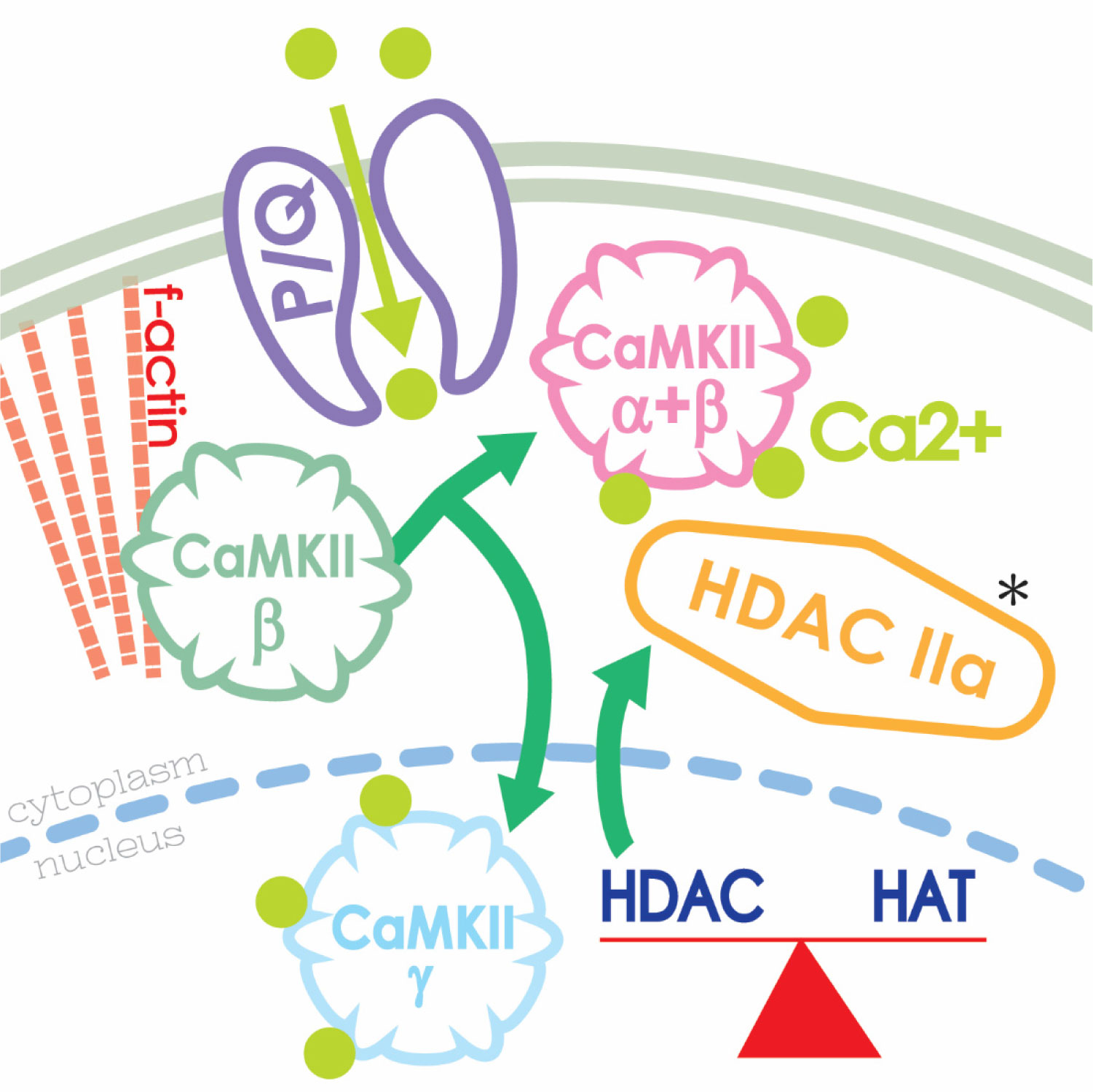
[59] | Urbano FJ, Bisagno V, Mahaffey S, et al. (2018) Class II histone deacetylases require P/Q-type Ca2+ channels and CaMKII to maintain gamma oscillations in the pedunculopontine nucleus. Nature Sci Rep 8: 13156. |
[60] | Urbano FJ, Bisagno V, Garcia-Rill E (2019) Neuroepigenetic control of gamma oscillations in the pedunculopontine nucleus: From HDACs to F-actin. Abstract #P-08-0375. International Brain Research Organization (IBRO) Meeting, Daegu, Korea. |
[61] |
Garcia-Rill E, Tackett AJ, Byrum SD, et al. (2019) Local and relayed effects of deep brain stimulation of the pedunculopontine nucleus. Brain Sci 9: E64. doi: 10.3390/brainsci9030064
![]() |
[62] |
Byrum S, Washam C, Tackett A, et al. (2019) Proteomic measures of gamma oscillations. Heliyon 5: e02265. doi: 10.1016/j.heliyon.2019.e02265
![]() |
[63] |
Garcia-Rill E, Charlesworth A, Heister D, et al. (2008) The developmental decrease in REM sleep: The role of transmitters and electrical coupling. Sleep 31: 673–690. doi: 10.1093/sleep/31.5.673
![]() |
[64] |
Choudhary C, Kumar C, Gnad F, et al. (2009) Lysine acetylation targets protein complexes and co-regulates major cellular functions. Science 325: 834–840. doi: 10.1126/science.1175371
![]() |
1. | A. Schrader, G. Crispatzu, S. Oberbeck, P. Mayer, S. Pützer, J. von Jan, E. Vasyutina, K. Warner, N. Weit, N. Pflug, T. Braun, E. I. Andersson, B. Yadav, A. Riabinska, B. Maurer, M. S. Ventura Ferreira, F. Beier, J. Altmüller, M. Lanasa, C. D. Herling, T. Haferlach, S. Stilgenbauer, G. Hopfinger, M. Peifer, T. H. Brümmendorf, P. Nürnberg, K. S. J. Elenitoba-Johnson, S. Zha, M. Hallek, R. Moriggl, H. C. Reinhardt, M.-H. Stern, S. Mustjoki, S. Newrzela, P. Frommolt, M. Herling, Actionable perturbations of damage responses by TCL1/ATM and epigenetic lesions form the basis of T-PLL, 2018, 9, 2041-1723, 10.1038/s41467-017-02688-6 |