Familiar fixes for a modern malady: a discussion on the possible cures of COVID-19

Amrit Krishna Mitra; Amrit Krishna Mitra

doi:10.3934/molsci.2020012

AIMS Molecular Science

2020, Volume 7, Issue 3:269-280. doi: 10.3934/molsci.2020012

Previous Article Next Article

Mini review

Familiar fixes for a modern malady: a discussion on the possible cures of COVID-19

Amrit Krishna Mitra ^,

Department of Chemistry, Government General Degree College, Singur, Hooghly, West Bengal, Pin: 712409, India

Received: 30 May 2020 Accepted: 13 July 2020 Published: 16 July 2020

Abstract
Full Text(HTML)
Download PDF

The SARS-CoV-2 virus emerged in December 2019 in Wuhan, China and then spread rapidly all over the world. Scientists are intensifying their research efforts in order to find antivirals specific to the virus and vaccines to treat or prevent COVID-19. Now, for a medicative cure for COVID-19, several drugs such as chloroquine, hydroxychloroquine, lopinavir, ritonavir, remdesivir and favipiravir are currently undergoing clinical studies. Convalescent plasma therapy and high dose of intravenous (IV) vitamin C have also been used to treat SARS-CoV-2 infections. This article outlines aspects related to several antiviral drugs and therapies which may be potentially effective against SARS-CoV-2.
- COVID-19,
- SARS-CoV-2,
- chloroquine,
- hydroxychloroquine,
- lopinavir,
- ritonavir,
- remdesivir,
- favipiravir,
- vitamin C,
- convalescent plasma
Citation: Amrit Krishna Mitra. Familiar fixes for a modern malady: a discussion on the possible cures of COVID-19[J]. AIMS Molecular Science, 2020, 7(3): 269-280. doi: 10.3934/molsci.2020012

Related Papers:

Abstract

The SARS-CoV-2 virus emerged in December 2019 in Wuhan, China and then spread rapidly all over the world. Scientists are intensifying their research efforts in order to find antivirals specific to the virus and vaccines to treat or prevent COVID-19. Now, for a medicative cure for COVID-19, several drugs such as chloroquine, hydroxychloroquine, lopinavir, ritonavir, remdesivir and favipiravir are currently undergoing clinical studies. Convalescent plasma therapy and high dose of intravenous (IV) vitamin C have also been used to treat SARS-CoV-2 infections. This article outlines aspects related to several antiviral drugs and therapies which may be potentially effective against SARS-CoV-2.

Acknowledgment

The author is extremely thankful to Mrs. Sayantani Mitra (Teacher, Department of English, Sushila Birla Girls' School, Kolkata, India), for her constant support in reviewing the manuscript.

Conflict of interest

The author declares no conflict of interest in this manuscript.

References

[1]	Andersen KG, Rambaut A, Lipkin WI, et al. (2020) The proximal origin of SARS-CoV-2. Nat Med 26: 450-452. doi: 10.1038/s41591-020-0820-9
[2]	Wu F, Zhao S, Yu B, et al. (2020) A new coronavirus associated with human respiratory disease in China. Nature 579: 265-269. doi: 10.1038/s41586-020-2008-3
[3]	Wang LF, Shi Z, Zhang S, et al. (2006) Review of bats and SARS. Emerg Infect Dis 12: 1834-1840. doi: 10.3201/eid1212.060401
[4]	Chen N, Zhou M, Dong X, et al. (2020) Epidemiological and clinical characteristics of 99 cases of 2019 novel coronavirus pneumonia in Wuhan, China: a descriptive study. Lancet 395: 507-513. doi: 10.1016/S0140-6736(20)30211-7
[5]	Huang C, Wang Y, Li X, et al. (2020) Clinical features of patients infected with 2019 novel coronavirus in Wuhan, China. Lancet 395: 497-506. doi: 10.1016/S0140-6736(20)30183-5
[6]	To KF, Tong JH, Chan PK, et al. (2004) Tissue and cellular tropism of the coronavirus associated with severe acute respiratory syndrome: an in-situ hybridization study of fatal cases. J Pathol 202: 157-163. doi: 10.1002/path.1510
[7]	Sungnak W, Huang N, Bécavin C, et al. (2020) SARS-CoV-2 entry factors are highly expressed in nasal epithelial cells together with innate immune genes. Nat Med 26: 681-687. doi: 10.1038/s41591-020-0868-6
[8]	Letko M, Marzi A, Munster V (2020) Functional assessment of cell entry and receptor usage for SARS-CoV-2 and other lineage B betacoronaviruses. Nat Microbiol 5: 562-569. doi: 10.1038/s41564-020-0688-y
[9]	Hoffmann M, Kleine-Weber H, Schroeder S, et al. (2020) SARS-CoV-2 Cell Entry Depends on ACE2 and TMPRSS2 and Is Blocked by a Clinically Proven Protease Inhibitor. Cell 181: 271-280. doi: 10.1016/j.cell.2020.02.052
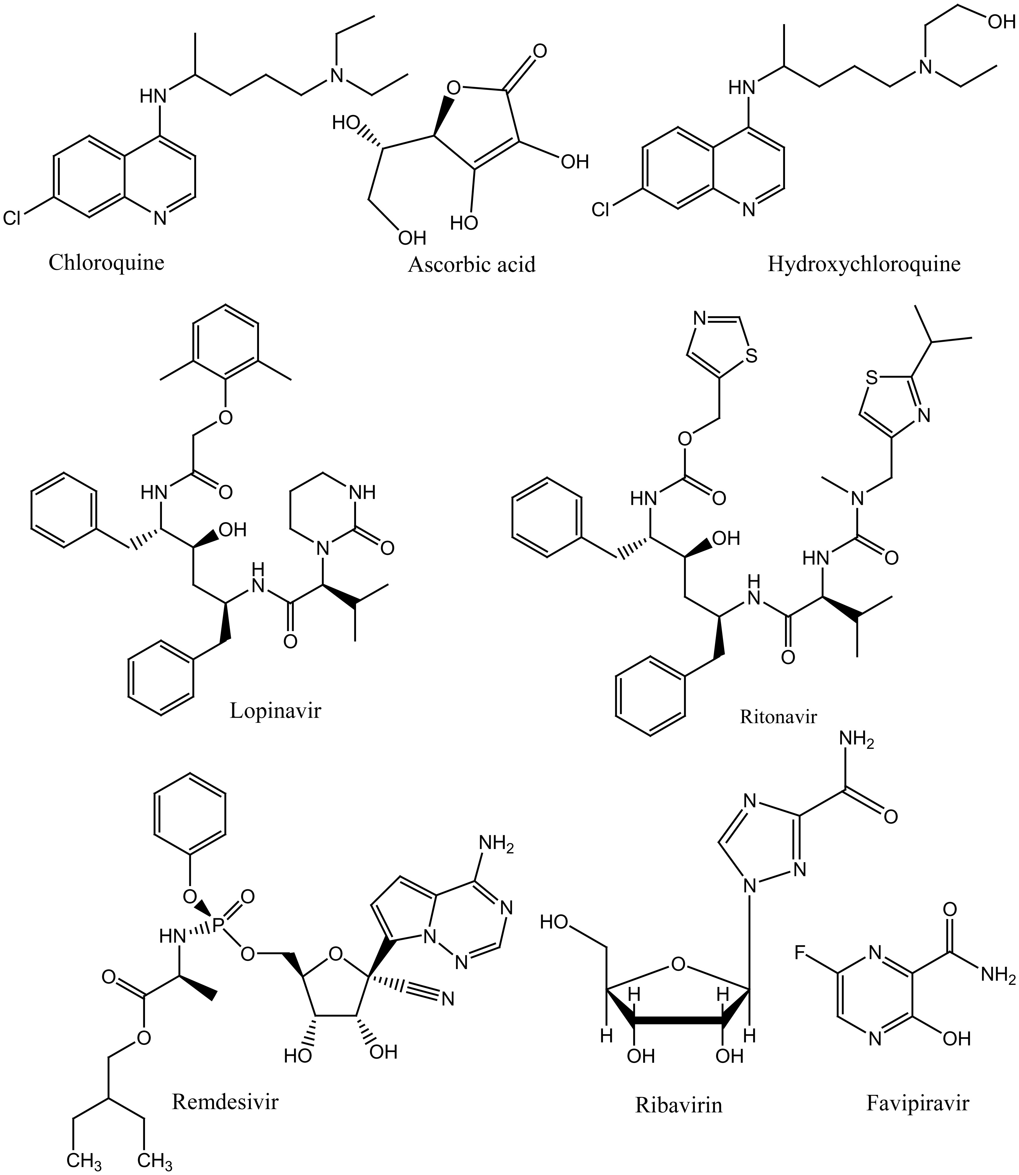
[10]	Chhikara BS, Rathi B, Singh J, et al. (2020) Corona virus SARS-CoV-2 disease COVID-19: Infection, prevention and clinical advances of the prospective chemical drug therapeutics. Chem Biol Lett 7: 63-72.
[11]	Eastman RT, Roth JS, Brimacombe KR, et al. (2020) Remdesivir: A Review of Its Discovery and Development Leading to Emergency Use Authorization for Treatment of COVID-19. ACS Cent Sci 6: 672-683. doi: 10.1021/acscentsci.0c00489
[12]	Keyaerts E, Vijgen L, Maes P, et al. (2004) In vitro inhibition of severe acute respiratory syndrome coronavirus by chloroquine. Biochem Biophys Res Commun 323: 264-268. doi: 10.1016/j.bbrc.2004.08.085
[13]	Gupta R, Ghosh A, Singh AK, et al. (2020) Clinical considerations for patients with diabetes in times of COVID-19 epidemic. Diabetes Metab Syndrome Clin Res Rev 14: 211-212. doi: 10.1016/j.dsx.2020.03.002
[14]	Morse JS, Lalonde T, Xu S, et al. (2020) Learning from the past: possible urgent prevention and treatment options for severe acute respiratory infections caused by 2019-nCoV. Chembiochem 21: 730-738. doi: 10.1002/cbic.202000047
[15]	Lai CC, Shih TP, Ko WC, et al. (2020) Severe acute respiratory syndrome coronavirus 2 (SARS-CoV-2) and coronavirus disease-2019 (COVID-19): The epidemic and the challenges. Int J Antimicrob Agents 55: 105924. doi: 10.1016/j.ijantimicag.2020.105924
[16]	Wang LS, Wang YR, Ye DW, et al. (2020) A review of the 2019 Novel Coronavirus (COVID-19) based on current evidence. Int J Antimicrob Agents 55: 105948. doi: 10.1016/j.ijantimicag.2020.105948
[17]	Lai CC, Liu YH, Wang CY, et al. (2020) Asymptomatic carrier state, acute respiratory disease, and pneumonia due to severe acute respiratory syndrome coronavirus 2 (SARS-CoV-2): facts and myths. J Microbiol Immunol Infect 4: 30040-30042.
[18]	Lu H (2020) Drug treatment options for the 2019-new coronavirus (2019-nCoV). Biosci Trends 14: 69-71. doi: 10.5582/bst.2020.01020
[19]	Gautret P, Lagier JC, Parola P, et al. (2020) Hydroxychloroquine and azithromycin as a treatment of COVID-19: results of an open-label non-randomized clinical trial. Int J Antimicrob Agents 105949.
[20]	Amrane S, Tissot-Dupont H, Doudier B, et al. (2020) Rapid viral diagnosis and ambulatory management of suspected COVID-19 cases presenting at the infectious diseases referral hospital in Marseille, France, - January 31st to March 1st, 2020: A respiratory virus snapshot. Travel Med Infect Dis 101632.
[21]	Chu CM, Cheng VC, Hung IF, et al. (2004) HKU/UCH SARS Study Group. Role of lopinavir/ ritonavir in the treatment of SARS: initial virological and clinical findings. Thorax 59: 252-256. doi: 10.1136/thorax.2003.012658
[22]	Snell NJ (2001) Ribavirin--current status of a broad spectrum antiviral agent. Expert Opin Pharmacother 2: 1317-1324. doi: 10.1517/14656566.2.8.1317
[23]	Vastag B (2003) Old drugs for a new bug. JAMA 290: 1695-1696. doi: 10.1001/jama.290.12.1569-a
[24]	Zhang L, Lin D, Sun X, et al. (2020) Crystal structure of SARS-CoV-2 main protease provides a basis for design of improved alpha-ketoamide inhibitors. Science 368: 409-412. doi: 10.1126/science.abb3405
[25]	Cao B, Wang Y, Wen D, et al. (2020) A Trial of Lopinavir–Ritonavir in Adults Hospitalized with Severe Covid-19. N Engl J Med 382: 1787-1799. doi: 10.1056/NEJMoa2001282
[26]	Deval J (2009) Antimicrobial strategies: inhibition of viral polymerases by 3′-hydroxyl nucleosides. Drugs 69: 151-166. doi: 10.2165/00003495-200969020-00002
[27]	Wang M, Cao R, Zhang L, et al. (2020) Remdesivir and chloroquine effectively inhibit the recently emerged novel coronavirus (2019-nCoV) in vitro. Cell Res 30: 269-271. doi: 10.1038/s41422-020-0282-0
[28]	ClinicalTrials.gov Mild/Moderate 2019-nCoV Remdesivir RCT. Available from: https://clinicaltrials.gov/ct2/show/NCT04252664.
[29]	ClinicalTrials.gov Severe 2019-nCoV Remdesivir RCT. Available from: https://clinicaltrials.gov/ct2/show/NCT04257656.
[30]	Holshue ML, DeBolt C, Lindquist S, et al. (2020) First Case of 2019 Novel Coronavirus in the United States. N Engl J Med 382: 929-936. doi: 10.1056/NEJMoa2001191
[31]	Delang L, Abdelnabi R, Neyts J (2018) Favipiravir as a potential countermeasure against neglected and emerging RNA viruses. Antivir Res 153: 85-94. doi: 10.1016/j.antiviral.2018.03.003
[32]	Dong L, Hu S, Gao J (2020) Discovering drugs to treat coronavirus disease 2019 (COVID-19). Drug Discov Ther 14: 58-60. doi: 10.5582/ddt.2020.01012
[33]	Lu H (2020) Drug Treatment Options for the 2019-new Coronavirus (2019-nCoV). Biosci Trends 14: 69-71. doi: 10.5582/bst.2020.01020
[34]	Coomes EA, Haghbayan H (2020) Favipiravir, an antiviral for COVID-19? J Antimicrob Chemother 75: 2013-2014. doi: 10.1093/jac/dkaa171
[35]	Seneviratne SL, Abeysuriya V, Mel SD, et al. (2020) Favipiravir in Covid-19. IJPSAT 19: 143-145.
[36]	Cheng Y, Wong R, Soo YOY, et al. (2005) Use of convalescent plasma therapy in SARS patients in Hong Kong. Eur J Clin Microbiol Infect Dis 24: 44-46. doi: 10.1007/s10096-004-1271-9
[37]	Zhou B, Zhong N, Guan N (2007) Treatment with convalescent plasma for influenza A (H5N1) infection. N Engl J Med 357: 1450-1451. doi: 10.1056/NEJMc070359
[38]	Lee PI, Hsueh PR (2020) Emerging threats from zoonotic coronaviruses-from SARS and MERS to 2019-nCoV. J Microbiol Immunol Infect 53: 365-367. doi: 10.1016/j.jmii.2020.02.001
[39]	Chen L, Xiong J, Bao L, et al. (2020) Convalescent plasma as a potential therapy for COVID-19. Lancet Infect Dis 20: 398-400. doi: 10.1016/S1473-3099(20)30141-9
[40]	Casadevall A, Joyner MJ, Pirofski LA (2020) A Randomized Trial of Convalescent Plasma for COVID-19—Potentially Hopeful Signals. JAMA E1-E3.
[41]	Chen N, Zhou M, Dong X, et al. (2020) Epidemiological and clinical characteristics of 99 cases of 2019 novel coronavirus pneumonia in Wuhan, China: a descriptive study. Lancet 395: 507-513. doi: 10.1016/S0140-6736(20)30211-7
[42]	Kindler E, Thiel V (2016) SARS-CoV and IFN: Too Little, Too Late. Cell Host Microbe 19: 139-141. doi: 10.1016/j.chom.2016.01.012
[43]	Ngo B, Van Ripper JM, Cantley LC, et al. (2019) Targeting cancer vulnerabilities with high-dose vitamin C. Nat Rev Cancer 19: 271-282. doi: 10.1038/s41568-019-0135-7
[44]	Yun J, Mullarky E, Lu C, et al. (2015) Vitamin C selectively kills KRAS and BRAF mutant colorectal cancer cells by targeting GAPDH. Science 350: 1391-1396. doi: 10.1126/science.aaa5004
[45]	Cummings M, Sarveswaran J, Homer-Vanniasinkam S, et al. (2014) Glyceraldehyde-3-phosphate dehydrogenase is an inappropriate housekeeping gene for normalising gene expression in sepsis. Inflammation 37: 1889-1894. doi: 10.1007/s10753-014-9920-3
[46]	Kashiouris MG, L'Heureux M, Cable CA, et al. (2020) The Emerging Role of Vitamin C as a Treatment for Sepsis. Nutrients 12: 292. doi: 10.3390/nu12020292
[47]	Cheng RZ (2020) Can early and high intravenous dose of vitamin C prevent and treat coronavirus disease 2019 (COVID-19)? Med Drug Discov 5: 100028. doi: 10.1016/j.medidd.2020.100028
[48]	Shanghai Expert Panel. Available from: http://mp.weixin.qq.com/s?__biz=MzA3Nzk5Mzc5MQ==&mid=2653620168&idx=1&sn=2352823b79a3cc42e48229a0c38f65e0&chksm=84962598b3e1ac8effb763e3ddb4858435dc7aa947a8f41790e8df2bca34c20e6ffea64cd191#rd.
[49]	Hemilä H, Chalker E (2019) Vitamin C can shorten the length of stay in the ICU: a meta-analysis. Nutrients 708: 1-30.
[50]	High-dose vitamin C (PDQ®)–Health professional version. National Cancer Institute. Available from: https://www.cancer.gov/about-cancer/treatment/cam/hp/vitamin-c-pdq.

Reader Comments

your name:*

Email:*
© 2020 the Author(s), licensee AIMS Press. This is an open access article distributed under the terms of the Creative Commons Attribution License (http://creativecommons.org/licenses/by/4.0)