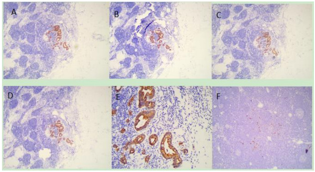
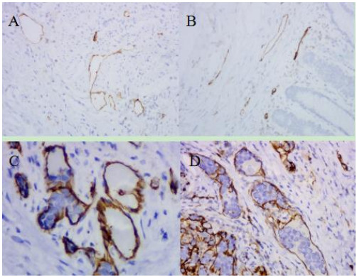
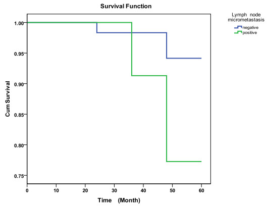
To investigate the significance of lymph node micrometastasis in T1N0 early gastric cancer. Lymph node micrometastasis may be a key mechanism in the recurrent T1N0 EGC patients after surgical treatment. It's unknow whether it is safe to leave the lymph nodes with micrometastasis untreated after ESD. A total of 106 T1N0 EGC patients were enrolled in this study. Immunohistochemical technique with CAM5.2 was employed to detect lymph node micrometastasis, and Immunohistochemical with D2-40 was used to detect the lymphatic vessels. Prognostic significance of lymph node micrometastasis and the relationship of lymph nodes micrometastasis with Clinicopathological features were analyzed. Twenty-two of the 106 T1N0 EGC cases were detected with lymph nodes micrometastasis, with the detection rate of 20.8%. The median survival time of the group with positive lymph nodes micrometastasis was lower than that of the group with negative micrometastasis, 48 vs 60 months. The incidence of lymph nodes micrometastasis in submucosal T1N0 EGC was 23.9%, while no micrometastasis was found in the mucosal T1N0 EGC. Of all the 30 cases according with the expanded ESD indications, six patients were found with lymph nodes micrometastasis. The occurrence of lymph node micrometastasis was common in T1N0 EGC. The cases with positive lymph nodes micrometastasis showed a lower median survival time than those with negative micrometastasis. lymph nodes micrometastasis incidence was higher in the submucosal ECG than in the mucosal ECG. lymph nodes micrometastasis was also found in the cases according to the expanded ESD indications.
Citation: Guochun Lou, Jie Dong, Jing Du, Wanyuan Chen, Xianglei He. Clinical significance of lymph node micrometastasis in T1N0 early gastric cancer[J]. Mathematical Biosciences and Engineering, 2020, 17(4): 3252-3259. doi: 10.3934/mbe.2020185
To investigate the significance of lymph node micrometastasis in T1N0 early gastric cancer. Lymph node micrometastasis may be a key mechanism in the recurrent T1N0 EGC patients after surgical treatment. It's unknow whether it is safe to leave the lymph nodes with micrometastasis untreated after ESD. A total of 106 T1N0 EGC patients were enrolled in this study. Immunohistochemical technique with CAM5.2 was employed to detect lymph node micrometastasis, and Immunohistochemical with D2-40 was used to detect the lymphatic vessels. Prognostic significance of lymph node micrometastasis and the relationship of lymph nodes micrometastasis with Clinicopathological features were analyzed. Twenty-two of the 106 T1N0 EGC cases were detected with lymph nodes micrometastasis, with the detection rate of 20.8%. The median survival time of the group with positive lymph nodes micrometastasis was lower than that of the group with negative micrometastasis, 48 vs 60 months. The incidence of lymph nodes micrometastasis in submucosal T1N0 EGC was 23.9%, while no micrometastasis was found in the mucosal T1N0 EGC. Of all the 30 cases according with the expanded ESD indications, six patients were found with lymph nodes micrometastasis. The occurrence of lymph node micrometastasis was common in T1N0 EGC. The cases with positive lymph nodes micrometastasis showed a lower median survival time than those with negative micrometastasis. lymph nodes micrometastasis incidence was higher in the submucosal ECG than in the mucosal ECG. lymph nodes micrometastasis was also found in the cases according to the expanded ESD indications.

| [1] |
J. Ferlay, H. R. Shin, F. Bray, D. Forman, C. Mathers, D. M. Parkin, Estimates of worldwide burden of cancer in 2008: GLOBOCAN 2008, Int. J. Cancer, 127(2010), 2893-2917. doi: 10.1002/ijc.25516

|
| [2] |
W. Tamura, N. Fukami, Early gastric cancer and dysplasia, Gastroint. Endosc. Clin. North Am., 23(2013), 77-94. doi: 10.1016/j.giec.2012.10.011
|
| [3] | J. J. Kim, K. Y. Song, H. Hur, J. I. Hur, S. M. Park, C. H. Park, Lymph node micrometastasis in node negative early gastric cancer, Eur. J. Surg. Oncol., 35(2009), 0-414. |
| [4] |
C. G. Liu, P. Lu, Y. Lu, R. S. Zhang, F. Jin, H. M. Xu, Relationship between preoperative clinicopathologic characteristics and lymph node metastasis in early gastric cancer, Chin. J. Cancer Res., 19(2007), 89-93. doi: 10.1007/s11670-007-0089-2
|
| [5] |
L. Cao, X. Hu, Y. Zhang, G. Huang, Adverse prognosis of clustered-cell versus single-cell micrometastases in pN0 early gastric cancer, J. Surg. Oncol., 103(2011), 53-56. doi: 10.1002/jso.21755
|
| [6] | H. Sonoda, K. Yamamoto, R. Kushima, Detection of lymph node micrometastasis in pN0 early gastric cancer: Efficacy of duplex RT-PCR with MUC2 and TFF1 in mucosal cancer, Oncol. Rep., 16(2006), 411-416. |
| [7] | Y. Maehara, T. Oshiro, K. Endo, H. Baba, S. Oda, Y. Ichiyoshi, Clinical significance of occult micrometastasis in lymph nodes from patients with early gastric cancer who died of recurrence, Surgery, 119(1996), 0-402. |
| [8] | H. Saito, T. D. Osaki, T. Sakamoto, S. Kanaji, S. Ohro, S. Tatebe, Recurrence in early gastric cancer--presence of micrometastasis in lymph node of node negative early gastric cancer patient with recurrence, Hepato Gastroenterol., 54(2007), 620-624. |
| [9] | N. Weidner, Intratumor microvessel density as a prognostic factor in cancer, Am. J. Pathol., 147(1995), 9-19. |
| [10] |
J. Cai, M. Ikeguchi, M. Maeta, Micrometastasis in lymph nodes and microinvasion of the muscularis propria in primary lesions of submucosal gastric cancer, Surgery, 127 (2000), 32-39. doi: 10.1067/msy.2000.100881
|
| [11] |
Y. Ikeda, M. Mori, K. Kajiyama, Y. Haraguchi, O. Sasaki, K. Sugimachi, Immunohistochemical expression of tenascin in normal stomach tissue, gastric carcinomas and gastric carcinoma in lymph nodes, Brit. J. Cancer, 72(1995), 189-192. doi: 10.1038/bjc.1995.301
|
| [12] | J. H. Cai, J. Liu, M. Ikeguch, Q. H. Yan, N. Kaibara, Clinical significance of micrometastasis in lymph nodes and microinvasion in primary lesion in submucosal gastric cancer, Zhonghua Wai Ke Za Zhi, 43(2005), 161-165. |
| [13] |
B. Valeria, R. Luca, E. Bonetti, Immunohistochemical assessment of lymphovascular invasion in stage I colorectal carcinoma: prognostic relevance and correlation with nodal micrometastases, Am. J. Surg. Path., 36(2012), 66-72. doi: 10.1097/PAS.0b013e31822d3008
|
| [14] |
M. Ishii, M. Ota, S. Saito, Y. Kinugasa, S. Akamoto, I. Ito, Lymphatic vessel invasion detected by monoclonal antibody D2-40 as a predictor of lymph node metastasis in T1 colorectal cancer, Int. J. Color. Dis., 24(2009), 1069-1074. doi: 10.1007/s00384-009-0699-x
|
| [15] |
A. A. Spycha, D. Murawa, K. Korski, The clinical importance of micrometastases within the lymphatic system in patients after total gastrectomy, Rep. Pract. Oncol. Radioth., 16(2011), 232-236. doi: 10.1016/j.rpor.2011.08.002
|
| [16] |
J. Rudno-Rudzinska, W. Kielan, Z. Grzebieniak, P. Dziegiel, P. Donizy, G. Mazur, High density of peritumoral lymphatic vessels measured by D2-40/podoplanin and LYVE-1 expression in gastric cancer patients: An excellent prognostic indicator or a false friend, Gastr. Cancer, 16(2013), 513-520. doi: 10.1007/s10120-012-0216-8
|
| [17] |
D. Paweł, J. Dembowski, K. Paweł, S. Tomasz, R. Zdrojowy, The clinical significance of lymphangiogenesis in renal cell carcinoma, Med. Sci. Monit., 19(2013), 606-611. doi: 10.12659/MSM.883981
|
| [18] |
Y. Xiong, L. P. Cao, H. L. Rao, M. Y. Cai, L. Z. Liang, J. H. Liu, Clinical significance of peritumoral lymphatic vessel density and lymphatic vessel invasion detected by D2-40 immunostaining in FIGO Ib1-IIa squamous cell cervical cancer, Cell. Tis. Res., 348(2012), 515-522. doi: 10.1007/s00441-012-1384-x
|
Figures(3) / Tables(2)

Guochun Lou, Jie Dong, Jing Du, Wanyuan Chen, Xianglei He. Clinical significance of lymph node micrometastasis in T1N0 early gastric cancer[J]. Mathematical Biosciences and Engineering, 2020, 17(4): 3252-3259. doi: 10.3934/mbe.2020185


 DownLoad: