Relative entropy minimization over Hilbert spaces via Robbins-Monro

1.   Introduction

In ^{[13,14,15,16,19]}, it was proposed that insight into a probability distribution, $\mu$, posed on a Hilbert space, $\mathcal{H}$, could be obtained by finding a best fit Gaussian approximation, $\nu$. This notion of best, or optimal, was with respect to the relative entropy, or Kullback-Leibler divergence:

Having a Gaussian approximation provides qualitative insight into $\mu$, as it provides a concrete notion of the mean and variance of the distribution. Additionally, this optimized distribution can be used in algorithms, such as random walk Metropolis, as a preconditioned proposal distribution to improve performance. Such a strategy can benefit a number of applications, including path space sampling for molecular dynamics and parameter estimation in statistical inverse problems.

Observe that in the definition of $\mathcal{R}$, (1.1), there is an asymmetry in the arguments. Were we to work with $\mathcal{R}(\mu||\nu)$, our optimal Gaussian would capture the first and second moments of $\mu$, and in some applications this is desirable. However, for a multimodal problem (consider a distribution with two well separated modes), this would be inadequate; our form attempts to match individual modes of the distribution by a Gaussian. For a recent review of the $\mathcal{R}(\nu||\mu)$ problem, see ^[4], where it is remarked that this choice of arguments is likely to underestimate the dispersion of the distribution of interest, $\mu$. The other ordering of arguments has been explored, in the finite dimensional case, in ^[2,3,10,18].

To be of computational use, it is necessary to have an algorithm that will converge to this optimal distribution. In ^[15], this was accomplished by first expressing $\nu = N(m, C(p))$, where $m$ is the mean and $p$ is a parameter inducing a well defined covariance operator, and then solving the problem,

over an admissible set. The optimization step itself was done using the Robbins-Monro algorithm (RM), ^[17], by seeking a root of the first variation of the relative entropy. While the numerical results of ^[15] were satisfactory, being consistent with theoretical expectations, no rigorous justification for the application of RM to the examples was given.

In this work, we emphasize the study and application of RM to potentially infinite dimensional problems. Indeed, following the framework of ^[15,16], we assume that $\mu$ is posed on the Borel $\sigma$-algebra of a separable Hilbert space $(\mathcal{H}, \left\langle {\bullet}, {\bullet}\right\rangle, \left \|{\bullet}\right\|)$. For simplicity, we will leave the covariance operator $C$ fixed, and only optimize over the mean, $m$. Even in this case, we are seeking $m\in \mathcal{H}$, a potentially infinite-dimensional space.

1.1.   Robbins-Monro

Given the objective function $f: \mathcal{H} \to \mathcal{H}$, assume that it has a root, $x_\star$. In our application to relative entropy, $f$ will be its first variation. Further, we assume that we can only observe a noisy version of $f$, $F: \mathcal{H} \times \chi\to \mathcal{H}$, such that for all $x \in \mathcal{H}$,

where $\mu_Z$ is the distribution associated with the random variable (r.v.) $Z$, taking values in the auxiliary space $\chi$. The naive Robbins-Monro algorithm is given by

where $Z_n \sim \mu_Z$, are independent and identically distributed (i.i.d.), and $a_n > 0$ is a carefully chosen sequence. Subject to assumptions on $f$, $F$, and the distribution $\mu_Z$, it is known that $X_n$ will converge to $x_\star$ almost surely (a.s.), in finite dimensions, ^[5,6,17]. Often, one needs to assume that $f$ grows at most linearly,

in order to apply the results in the aforementioned papers. The analysis in the finite dimensional case has been refined tremendously over the years, including an analysis based on continuous dynamical systems. We refer the reader to the books ^[1,8,11] and references therein.

1.2.   Trust regions and truncations

As noted, much of the analysis requires the regression function $f$ to have, at most, linear growth. Alternatively, an a priori assumption is sometimes made that the entire sequence generated by (1.4) stays in a bounded set. Both assumptions are limiting, though, in practice, one may find that the algorithms converge.

One way of overcoming these assumptions, while still ensuring convergence, is to introduce trust regions that the sequence $\{X_n\}$ is permitted to explore, along with a "truncation" which enforces the constraint. Such truncations distort (1.4) into

where $P_{n+1}$ is the projection keeping the sequence $\{X_n\}$ within the trust region. Projection algorithms are also discussed in ^[1,8,11].

We consider RM on a possibly infinite dimensional separable Hilbert space. This is of particular interest as, in the context of relative entropy optimization, we may be seeking a distribution in a Sobolev space associated with a PDE model. A general analysis of RM with truncations in Hilbert spaces can be found in ^[20]. The main purpose of this work is to adapt the analysis of ^[12] to the Hilbert space setting for two versions of the truncated problem. The motivation for this is that the analysis of ^[12] is quite straightforward, and it is instructive to see how it can be easily adapted to the infinite dimensional setting. The key modification in the proof is that results for Banach space valued martingales must be invoked. We also adapt the results to a version of the algorithm where there is prior knowledge on the location of the root. With these results in hand, we can then verify that the relative entropy minimization problem can be solved using RM.

1.2.1.   Fixed trust regions

In some problems, one may have a priori information on the root. For instance, we may know that $x_\star \in U_1$, some open bounded set. In this version of the truncated algorithm, we have two open bounded sets, $U_0\subsetneq U_1$, and $x_\star \in U_1$. Let $\sigma_0 = 0$ and $X_0 \in U_0$ be given, then (1.6) can be formulated as

We interpret $\tilde{X}_{n+1}$ as the proposed move, which is either accepted or rejected depending on whether or not it will remain in the trust region. If it is rejected, the algorithm restarts at $X_{0}^{(\sigma_n)}\in U_0$. The restart points, $\{X_{0}^{(\sigma_n)}\}$, may be random, or it may be that $X_{0}^{(\sigma_n)} = X_0$ is fixed. The essential property is that the algorithm will restart in the interior of the trust region, away from its boundary. The r.v. $\sigma_n$ counts the number of times a truncation has occurred. Algorithm (1.7) can now be expressed as

1.2.2.   Expanding trust regions

In the second version of truncated Robbins-Monro, define the sequence of open bounded sets, $U_{n}$ such that:

Again, letting $X_0 \in U_0$, $\sigma_0 = 0$, the algorithm is

A consequence of this formulation is that $X_n \in U_{\sigma_n}$ for all $n$. As before, the restart points may be random or fixed, and they are in $U_0$. This would appear superior to the fixed trust region algorithm, as it does not require knowledge of the sets. However, to guarantee convergence, global (in $\mathcal{H}$) assumptions on the regression function are required; see Assumption 2 below. (1.10) can written with $P_{n+1}$ as

1.3.   Outline

In Section 2, we state sufficient assumptions for which we are able to prove convergence in both the fixed and expanding trust region problems, and we also establish some preliminary results. In Section 3, we focus on the relative entropy minimization problem, and identify what assumptions must hold for convergence to be guaranteed. Examples are then presented in Section 4, and we conclude with remarks in Section 5.

2.   Convergence of Robbins-Monro

We first reformulate (1.8) and (1.15) in the more general form

where $\delta M_{n+1}$, the noise term, is

A natural filtration for this problem is $\mathcal{F}_n = \sigma(X_0, Z_1, \ldots, Z_n)$. $X_n$ is $\mathcal{F}_n$ measurable and the noise term can be expressed in terms of the filtration as $\delta M_{n+1} = F(X_n, Z_{n+1}) - \mathbb{E}[F(X_n, Z_{n+1})\mid \mathcal{F}_n]$.

We now state our main assumptions:

Assumption 1. $f$ has a zero, $x_\star$. In the case of the fixed trust region problem, there exist $R_0 < R_1$ such that

In the case of the expanding trust region problem, the open sets are defined as $U_n = B_{r_n}(0)$ with

These sets clearly satisfy (1.9).

Assumption 2. For any $0 < a < A$, there exists $\delta > 0$:

In the case of the fixed truncation, this inequality is restricted to $x\in U_1$. This is akin to a convexity condition on a functional $\mathcal{F}$ with $f = D\mathcal{F}$.

Assumption 3. $x\mapsto \mathbb{E}[\left \|{F(x, Z)}\right\|^2]$ is bounded on bounded sets, with the restriction to $U_1$ in the case of fixed trust regions.

Assumption 4. $a_n > 0$, $\sum a_n = \infty$, and $\sum a_n^2 < \infty$

Theorem 2.1. Under the above assumptions, for the fixed trust region problem, $X_n \to x_\star$ a.s. and $\sigma_n$ is a.s. finite.

Theorem 2.2. Under the above assumptions, for the expanding trust region problem, $X_n \to x_\star$ a.s. and $\sigma_n$ is a.s. finite.

Note the distinction between the assumptions in the two algorithms. In the fixed truncation algorithm, Assumptions 2 and 3 need only hold in the set $U_1$, while in the expanding truncation algorithm, they must hold in all of $\mathcal{H}$. While this would seem to be a weaker condition, it requires identification of the sets $U_0$ and $U_1$ for which the assumptions hold. Such sets may not be readily identifiable, as we will see in our examples.

We first need some additional information about $f$ and the noise sequence $\delta M_n$.

Lemma 2.1. Under Assumption 3, $f$ is bounded on $U_1$, for the fixed trust region problem, and on arbitrary bounded sets, for the expanding trust region problem.

Proof. Trivially,

and the results follows from the assumption.

Proposition 2.1. For the fixed trust region problem, let

Alternatively, in the expanding trust region problem, for $r > 0$, let

Under Assumptions 3 and 4, $M_n$ is a martingale, converging in $\mathcal{H}$, a.s.

Proof. The following argument holds in both the fixed and expanding trust region problems, with appropriate modifications. We present the expanding trust region case. The proof is broken up into 3 steps:

$1.$ Relying on Theorem 6 of ^[7] for Banach space valued martingales, it will be sufficient to show that $M_n$ is a martingale, uniformly bounded in $L^1(\mathbb{P})$.

$2.$ In the case of the expanding truncations,

Since both of these terms are bounded, independently of $i$, by Assumption 3 and Lemma 1, this is finite.

$3.$ Next, since $\{\delta M_i 1_{\|X_{i-1}-x_\star\|\leq r}\}$ is a martingale difference sequence, we can use the above estimate to obtain the uniform $L^2(\mathbb{P})$ bound,

Uniform boundedness in $L^2$, gives boundedness in $L^1$, and this implies a.s. convergence in $\mathcal{H}$.

2.1.   Finite truncations

In this section we prove results showing that only finitely many truncations will occur, in either the fixed or expanding trust region case. Recall that when a truncation occurs, the equivalent conditions hold: $P_{n+1}\neq 0$; $\sigma_{n+1} = \sigma_n+1$; and $\tilde{X}_{n+1}\notin U_1$ in the fixed trust region algorithm, while $\tilde{X}_{n+1}\notin U_{\sigma_n}$ in the expanding trust region case.

Lemma 2.2. In the fixed trust region algorithm, if Assumptions 1, 2, 3, and 4 hold, then the number of truncations is a.s. finite; a.s., there exists $N$, such that for all $n\geq N$, $\sigma_n = \sigma_N$.

Proof. We break the proof up into 7 steps:

1. Pick $\rho$ and $\rho'$ such that

Let $\bar f = \sup\|f(x)\|$, with the supremum over $U_1$; this bound exists by Lemma 1. Under Assumption 2, there exists $\delta > 0$ such that

Having fixed $\rho$, $\rho'$, $\bar f$, and $\delta$, take $\epsilon > 0$ such that:

Having fixed such an $\epsilon$, by the assumptions of this lemma and Proposition 1, a.s., there exists $n_{ \epsilon}$ such that for any $n, m\geq n_{ \epsilon}$, both

$2.$ Define the auxiliary sequence

Using (2.1), we can then write

By (2.7), for any $n \geq n_ \epsilon$,

$3.$ We will show $X_n' \in B_{\rho'}(x_\star)$ for all $n$ large enough. The significance of this is that if $n\geq n_ \epsilon$, and $X_n'\in B_{\rho'}(x_\star)$, then no truncation occurs. Indeed, using (2.6)

Consequently, $P_{n+1} = 0$, $X_{n+1} = \tilde{X}_{n+1}$, and $\sigma_{n+1} = \sigma_n$. Thus, establishing $X_n'\in B_{\rho'}(x_\star)$ will yield the result.

$4.$ Let

This corresponds to the the first truncation after $n_ \epsilon$. If the above set is empty, for that realization, no truncations occur after $n_ \epsilon$, and we are done. In such a case, we may take $N = n_ \epsilon$ in the statement of the lemma.

$5.$ We now prove by induction that in the case that (2.12) is finite, $X_n'\in B_{\rho'}(x_\star)$ for all $n\geq N$. First, note that $X_N \in B_{R_0}(x_\star)\subset B_{\rho}(x_\star)$. By (2.6) and (2.10),

Next, assume $X_{N}', X_{N+1}', \ldots, X_n'$ are all in $B_{\rho'}(x_\star)$. Using (2.11), we have that $P_{N+1} = \ldots = P_{n+1} = 0$ and $\sigma_{N} = \ldots = \sigma_{n} = \sigma_{n+1}$. Therefore,

We now consider two cases of (2.13) to conclude $\|X_{n+1}' - x_\star\| < \rho'$.

$6.$ In the first case, $\|X'_n - x_\star\|\leq R_0$. By Cauchy-Schwarz and (2.6)

In the second case, $R_0 < \|X'_n - x_\star\| < \rho'$. Dissecting the inner product term in (2.13) and using Assumption 2 and (2.10),

Conditions (2.6) and (2.10) yield the following upper and lower bounds:

Therefore, (2.5) applies and $\left\langle {X_{n}-x_\star}, {f(X_n)}\right\rangle\geq \delta$. Using this in (2.14), and condition (2.6),

Substituting this last estimate back into (2.13), and using (2.6),

This completes the inductive step.

$7.$ Since the auxiliary sequence remains in $B_{\rho'}(x_\star)$ for all $n\geq N > n_ \epsilon$, (2.11) ensures $\tilde X_{n+1}\in B_{R_1}(x_\star)$, $P_{n+1} = 0$, and $\sigma_{n+1} = \sigma_N$, a.s.

To obtain a similar result for the expanding trust region problem, we first relate the finiteness of the number of truncations with the sequence persisting in a bounded set.

Lemma 2.3. In the expanding trust region algorithm, if Assumptions 1, 3, and 4 hold, then the sequence remains in a set of the form $B_{R}(0)$ for some $R > 0$ if and only if the number of truncations is finite, a.s.

Proof. We break this proof into 4 steps:

$1.$ If the number of truncations is finite, then there exists $N$ such that for all $n\geq N$, $\sigma_n = \sigma_{N}$. Consequently, the proposed moves are always accepted, and $X_{n} \in U_{\sigma_{n}} = U_{\sigma_N}$ for all $n\geq N$. Since $X_n \in U_{\sigma_n}\subset U_{\sigma_N}$ for $n < N$, $X_n \in U_{\sigma_N}$ for all $n$. By Assumption 3, $B_R(0) = B_{r_{\sigma_N}}(0) = U_{\sigma_N}$ is the desired set.

$2.$ For the other direction, assume that there exists $R > 0$ such that $X_n \in B_R(0)$ for all $n$. Since the $r_n$ in (2.3) tend to infinity, there exists $N_1$, such that $R < R +1 < r_{N_1}$. Hence, for all $n\geq N_1$,

Let $\bar f = \sup \|f(x)\|$, with the supremum over $B_{R}(0)$. Let $\tilde{R}$ be sufficiently large such that $B_{R+1}(0)\subset B_{\tilde R}(x_\star)$. Lastly, using Proposition 1 and Assumption 4, a.s., there exists $N_2$, such that for all $n\geq N_2$

Since $X_n \in B_{R}(0) \subset B_{\tilde R}(x_\star)$, the indicator function in (2.16) is always one, and $\| a_{n} \delta M_{n}\| < 1/2$.

$3.$ Next, let

If the above set is empty, then $\sigma_n < \max\{N_1, N_2\}$ for all $n$, and the number of truncations is a.s. finite. In this case, the proof is complete.

$4.$ If the set in (2.17) is not empy, then $N < \infty$. Take $n\geq N$. As $X_n \in B_R(0)$, and since $n\geq \sigma_n\geq \max\{N_1, N_2\}$, (2.16) applies. Therefore,

Thus, $\tilde{X}_{n+1}\in B_{R+1}(0)\subset U_{N_1}$, $\sigma_n \geq N_1$, and $U_{N_1}\subset U_{\sigma_n}$. Therefore, $\tilde{X}_{n+1}\in U_{\sigma_n}$. No truncation occurs, and $\sigma_n = \sigma_{n+1}$. Since this holds for all $n\geq N$, $\sigma_n = \sigma_N$, and the number of truncations is a.s. finite.

Next, we establish that, subject to an additional assumption, the sequence remains in a bounded set; the finiteness of the truncations is then a corollary.

Lemma 2.4. In the expanding trust region algorithm, if Assumptions 1, 2, 3, and 4 hold, and for any $r > 0$, there a.s. exists $N < \infty$, such that for all $n \geq N$,

then $\{X_n\}$ remains in a bounded open set, a.s.

Proof. We break this proof into 7 steps:

$1.$ We begin by setting some constants for the rest of the proof. Fix $R > 0$ sufficiently large such that $B_{R}(x_\star)\supset U_0$. Next, let $\bar f = \sup {\|f(x)\|}$ with the supremum taken over $B_{R+2}(x_\star)$. Assumption 2 ensures there exists $\delta > 0$ such that

Having fixed $R$, $\bar f$, and $\delta$, take $\epsilon > 0$ such that:

By the assumptions of this lemma and Proposition 1 there exists, a.s., $n_ \epsilon\geq N$ such that for all $n\geq n_ \epsilon$,

$2.$ Define the modified sequence for $n \geq n_ \epsilon$ as

Using (2.1), we have the iteration

$3.$ Let

the first time after $n_ \epsilon$ that a truncation occurs.

If the above set is empty, no truncations occur after $n_ \epsilon$. In this case, $\sigma_n = \sigma_{n_ \epsilon}\leq n_ \epsilon < \infty$ for all $n \geq n_ \epsilon$. Therefore, for all $n\geq n_ \epsilon$, $X_n \in U_{\sigma_n}\subset U_{\sigma_{n_ \epsilon}}$. Since $U_{\sigma_n}\subset U_{\sigma_{n_ \epsilon}}$ for all $n < n_ \epsilon$ too, the proof is complete in this case.

$4.$ Now assume that $N < \infty$. We will show that $\{X_n'\}$ remains in $B_{R+1}(x_\star)$ for all $n\geq N$. Were this to hold, then for $n\geq N$,

having used (2.21) and (2.22). For $n < N$, $X_n \in U_{\sigma_n}\subset U_{\sigma_N} = B_{r_N}(0)$. Therefore, for all $n$, $X_n \in B_{\tilde{R}}(0)$ where $\tilde{R} = \max\{ r_N, \|x_\star\| + R+2\}$.

$5.$ We prove $X_n' \in B_{R+1}(x_\star)$ by induction. First, since $\epsilon < 1$ and $X_N \in U_{0}\subset B_R(x_\star)$,

Next, assume that $X_N', X_{N+1}', \ldots, X_n'$ are all in $B_{R+1}(x_\star)$. By (2.25), $X_n\in B_{R+2}(x_\star)$. Since $P_{n+1} 1_{\left \|{X_{n}- x_\star}\right\|\leq R+2} = 0$, we conclude $P_{n+1} = 0$. The modified iteration (2.23) simplifies to have

and

$6.$ We now consider two cases of (2.26). First, assume $\|X'_{n} - x_\star\|\leq R$. Then (2.26) can immediately be bounded as

where we have used condition (2.20) in the last inequality.

$7.$ Now consider the case $R < \|X'_{n} - x_\star\| < R+1$. Using (2.20), the inner product in (2.26) can first be bounded from below:

Next, using (2.20)

Therefore, $\tfrac{1}{2}R < \|X_n -x_\star\| < R+2$, so (2.19) ensures $\left\langle {X_{n}-x_\star}, {f(X_n)}\right\rangle\geq\delta$ and

Returning to (2.26), by (2.20),

This completes the proof of the inductive step in this second case, completing the proof.

Corollary 2.1. For the expanding trust region algorithm, if Assumptions 1, 2, 3, and 4 hold, then the number of truncations is a.s. finite.

Proof. The proof is by contradiction. We break the proof into 4 steps:

$1.$ Assuming that there are infinitely many truncations, Lemma 3 implies that the sequence cannot remain in a bounded set. Then, continuing to assume that Assumptions 1, 2, 3, and 4 hold, the only way for the conclusion of Lemma 4 to fail is if the assumption on $P_{n+1} 1_{\|X_n - x_\star\|\leq r }$ is false. Therefore, there exists $r > 0$ and a set of positive measure on which a subsequence, $P_{n_k+1} 1_{\|X_{n_k} - x_\star\|\leq r }\neq 0$. Hence $X_{n_k}\in B_{r}(x_\star)$, and $P_{n_k+1}\neq 0$. So truncations occur at these indices, and $\tilde{X}_{n_k+1} \not\in U_{\sigma_{n_k}}$.

$2.$ Let $\bar{f} = \sup \|f(x)\|$ with the supremum over the set $B_r(x_\star)$ and let $\epsilon > 0$ satisfy

By our assumptions of the lemma and Proposition 1, there exists $n_ \epsilon$ such that for all $n\geq n_ \epsilon$

Along the subsequence, for all $n_k\geq n_ \epsilon$,

$3.$ Furthermore, for $n_k \geq n_ \epsilon$:

where (2.27) has been used in the last inequality.

$4.$ By the definition of the $U_n$, there exists an index $M$ such that $U_{M}\supset B_{r+1}(x_\star)$. Let

This set is nonempty and $N < \infty$ since we have assumed there are infinitely many truncations. Let $n_k \geq N$. Then $\sigma_{n_k}\geq M$ and $U_{\sigma_{n_k}}\supset B_{r+1}(x_\star)$. But (2.30) then implies that $\tilde{X}_{n_k+1} \in U_{\sigma_{n_k}}$, and no truncation will occur; $P_{n_k+1} = 0$, providing the desired the contradiction.

2.2.   Proof of convergence

Using the above results, we are able to prove Theorems 2.1 and 2.2. Since the proofs are quite similar, we present the more complicated expanding trust region case.

Proof. We split this proof into 6 steps:

$1.$ First, by Corollary 1, only finitely many truncations occur. By Lemma 3, there exists $R > 0$ such that $X_n\in B_R(0)$ for all $n$. Consequently, there is an $r$ such that $X_n\in B_r(x_\star)$ for all $n$.

$2.$ Next, we fix constants. Let $\bar f = \sup \|f(x)\|$ with the supremum taken over $B_r(x_\star)$. Fix $\eta \in (0, 2R)$, and use Assumption 2 to determine $\delta > 0$ such that

Take $\epsilon > 0$ such that:

Having set $\epsilon$, we again appeal to Assumption 4 and Proposition 1 to find $n_ \epsilon$ such that for all $n\geq n_ \epsilon$:

$3.$ Define the auxiliary sequence,

Since there are only finitely many truncations, there exists $N\geq n_ \epsilon$, such that for all $n\geq N$, $P_{n+1} = 0$, as the truncations have ceased. Consequently, for $n\geq N$,

By (2.34) and (2.35), for $n\geq N$, $\|X_n - X_n'\|\leq \epsilon$. Since $\epsilon > 0$ may be arbitrarily small, it will be sufficient to prove $X_n'\to x_\star$.

$4.$ To obtain convergence of $X_n'$, we first examine $\|X_{n+1}'-x_\star\|$. For $n\geq N$,

Now consider two cases of this expression. First, assume $\|X_n' - x_\star\|\leq\eta$. In this case, using (2.33),

where $B > 0$ is a constant depending only on $R$ and $\bar f$. For $\|X_n' - x_\star\| > \eta$, using (2.33)

By (2.33),

Since $\|X_n - x_\star\| < r$ too, (2.32) and (2.39) yield the estimate

Thus, in this regime, using (2.33),

where $A > 0$ is a constant depending only on $\delta$.

Combining estimates (2.38) and (2.40), we can write for $n\geq N$

$5.$ We now show that $\|X_n' - x_\star\|\leq \eta$ i.o. The argument is by contradiction. Let $M\geq N$ be such that for all $n\geq M$, $\|X_n' - x_\star\| > \eta$. For such $n$,

Using Assumption 4 and taking $n\to \infty$, we obtain a contradiction.

$6.$ Finally, we prove convergence of $X_n'\to x_\star$. Since $X_n'\in B_{\eta}(x_\star)$ i.o., let

For $n\geq N'$, we can then define

For all such $n$, $\varphi(n)\leq n$, and $X_{\varphi(n)}'\in B_\eta(x_\star)$.

We claim that for $n\geq N'$,

First, if $n = \varphi(n)$, this trivially holds in (2.41). Suppose now that $n > \varphi(n)$. Then for $i = \varphi(n)+1, \varphi(n)+2, \ldots n$, $\|X_{i}' - x_\star\| > \eta$. Consequently,

As $\varphi(n)\to \infty$,

Since $\eta$ may be arbitrarily small, we conclude that

completing the proof.

3.   Minimization of relative entropy

Recall from the introduction that our distribution of interest, $\mu$, is posed on the Borel subsets of Hilbert space $\mathcal{H}$. We assume that $\mu \ll \mu_0$, where $\mu_0 = N(m_0, C_0)$ is some reference Gaussian. Thus, we write

where $\Phi_\nu: X\to \mathbb{R}$, $X$ a Banach space, a subspace of $\mathcal{H}$, of full measure with respect to $\mu_0$, a Gaussian on $\mathcal{H}$, assumed to be continuous. $Z_\mu = \mathbb{E}^{\mu_0}[\exp\left\{{-\Phi(u)}\right\}]\in (0, \infty)$ is the partition function ensuring we have a probability measure.

Let $\nu = N(m, C)$, be another Gaussian, equivalent to $\mu_0$, such that we can write

Assuming that $\nu \ll \mu$, we can write

The assumption that $\nu \ll \mu$ implies that $\nu$ and $\mu$ are equivalent measures. As was proven in ^[16], if $\mathcal{A}$ is a set of Gaussian measures, closed under weak convergence, such that at least one element of $\mathcal{A}$ is absolutely continuous with respect to $\mu$, then any minimizing sequence over $\mathcal{A}$ will have a weak subsequential limit.

If we assume, for this work, that $C = C_0$, then, by the Cameron-Martin formula (see ^[9]),

Here, $\left\langle {\bullet}, {\bullet}\right\rangle_{ \mathcal{H}^1}$ and $\|\bullet\|_{ \mathcal{H}^1}$ are the inner product and norms of the Cameron-Martin Hilbert space, denoted $\mathcal{H}^1$,

Convergence to the minimizer will be established in $\mathcal{H}^1$, and $\mathcal{H}^1$ will be the relevant Hilbert space in our application of Theorems 2.1 and 2.2 to this problem.

Letting $\nu_0 = N(0, C_0)$ and $v\sim \nu_0$, we can then rewrite (3.3) as

The Euler-Lagrange equation associated with (3.6), and the second variation, are:

3.1.   Application of Robbins-Monro

In ^[15], it was suggested that rather than try to find a root of (3.7), the equation first be preconditioned by multiplying by $C_0$,

and a root of this mapping is sought, instead. Defining

The Robbins-Monro formulation is then

with $v_n \sim \nu_0$, i.i.d.

We thus have

Theorem 3.1. Assume:

● There exists $\nu = N(m, C_0)\sim \mu_0$ such that $\nu\ll\mu$.

● $\Phi_\mu'$ and $\Phi_\mu''$ exist for all $u \in \mathcal{H}^1$.

● There exists $m_\star$, a local minimizer of $J$, such that $J'(m_\star) = 0$.

● The mapping

is bounded on bounded subsets of $\mathcal{H}^1$.

● There exists a convex neighborhood $U_\star$ of $m_\star$ and a constant $\alpha > 0$, such that for all $m\in U_\star$, for all $u \in \mathcal{H}^1$,

Then, choosing $a_n$ according to Assumption 4,

● If the subset $U_\star$ can be taken to be all of $\mathcal{H}^1$, for the expanding truncation algorithm, $m_n \to m_\star$ a.s. in $\mathcal{H}^1$.

● If the subset $U_\star$ is not all of $\mathcal{H}^1$, then, taking $U_1$ to be a bounded (in $\mathcal{H}^1$) convex subset of $U_\star$, with $m_\star \in U_1$, and $U_0$ any subset of $U_1$ such that there exist $R_0 < R_1$ with

for the fixed truncation algorithm, $m_n\to m_\star$ a.s. in $\mathcal{H}^1$.

Proof. We split the proof into 2 steps:

$1.$ By the assumptions of the theorem, we clearly satisfy Assumptions 1 and 4. To satisfy Assumption 3, we observe that

This is bounded on bounded subsets of $\mathcal{H}^1$.

$2.$ Per the convexity assumption, (3.14), implies Assumption 2, since, by the mean value theorem in function spaces,

where $\tilde m$ is some intermediate point between $m$ and $m_\star$. This completes the proof.

While condition (3.14) is sufficient to obtain convexity, other conditions are possible. For instance, suppose there is a convex open set $U_\star$ containing $m_\star$ and constant $\theta\in [0, 1)$, such that for all $m \in U_\star$,

where $\lambda_1$ is the principal eigenvalue of $C_0$. Then this would also imply Assumption 2, since

We mention (3.15) as there may be cases, shown below, for which the operator $\mathbb{E}^{\nu_0}[\Phi''_\mu(v+ m)]$ is obviously nonnegative.

4.   Examples

To apply the Robbins-Monro algorithm to the relative entropy minimization problem, the $\Phi_\mu$ functional of interest must be examined. In this section we present a few examples, based on those presented in ^[15], and examine when the assumptions hold. The one outstanding assumption that we must make is that, a priori, $\mu_0$ is an equivalent measure to $\mu$.

4.1.   Scalar problem

Taking $\mu_0 = N(0, 1)$, the standard unit Gaussian, let $V: \mathbb{R} \to \mathbb{R}$ be a smooth function such that

is a probability measure on $\mathbb{R}$. For these scalar cases, we use $x$ in place of $v$. In the above framework,

and $\xi\sim N(0, 1) = \nu_0 = \mu_0$.

4.1.1.   Globally convex case

Consider the case that

In this case

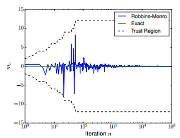
Since $\mathbb{E}[\Phi''_\mu(x+\xi)] \geq 4 { \epsilon^{-1}}$, all of our assumptions are satisfied and the expanding truncation algorithm will converge to the unique root at $x_\star = 0$ a.s. See Figure 1 for an example of the convergence at $\epsilon = 0.1$, $U_{n} = (-n -1, n+1)$, and always restarting at $0.5$.

We refer to this as a "globally convex'' problem since $\mathcal{R}$ is globally convex about the minimizer.

4.1.2.   Locally convex case

In contrast to the above problem, some mimizers are only "locally'' convex. Consider the case the double well potential

Now, the expressions for RM are

In this case, $f(x)$ vanishes at $0$ and $\pm \sqrt{1- \epsilon}$, and $J''$ changes sign from positive to negative when $x$ enters $({-\sqrt{(1- \epsilon)/3}, \sqrt{({1- \epsilon})/{3}}})$. We must therefore restrict to a fixed trust region if we want to ensure convergence to either of $\pm\sqrt{1- \epsilon}$.

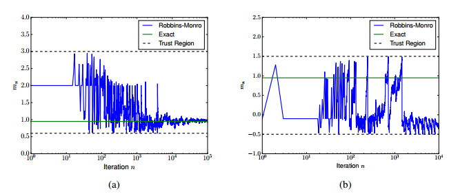
We ran the problem at $\epsilon = 0.1$ in two cases. In the first case, $U_1 = (0.6, 3.0)$ and the process always restarts at $2$. This guarantees convergence since the second variation will be strictly postive. In the second case, $U_1 = (-0.5, 1.5)$, and the process always restarts at $-0.1$. Now, the second variation can change sign. The results of these two experiments appear in Figure 2. For some random number sequences the algorithm still converged to $\sqrt{1- \epsilon}$, even with the poor choice of trust region.

4.2.   Path space problem

Take $\mu_0 = N(m_0(t), C_0)$, with

equipped with Dirichlet boundary conditions on $\mathcal{H} = L^2(0, 1)$.^* In this case the Cameron-Martin space $\mathcal{H}^1 = H^1_0(0, 1)$, the standard Sobolev space equipped with the Dirichlet norm. Let us assume $m_0 \in H^1(0, 1)$, taking values in $\mathbb{R}^d$.

^* This is the covariance of the standard unit Brownian bridge, $Y_t = B_t - t B_1$.

Consider the path space distribution on $L^2(0, 1)$, induced by

where $V: \mathbb{R}^d\to \mathbb{R}$ is a smooth function. We assume that $V$ is such that this probability distribution exists and that $\mu \sim \mu_0$, our reference measure.

We thus seek an $\mathbb{R}^d$ valued function $m(t) \in H^1(0, 1)$ for our Gaussian approximation of $\mu$, satisfying the boundary conditions

For simplicity, take $m_0 = (1-t)m_- + t m_+$, the linear interpolant between $m_\pm$. As above, we work in the shifted coordinated $x(t) = m(t) - m_0(t)\in H^1_0(0, 1)$.

Given a path $v(t)\in H^1_0$, by the Sobolev embedding, $v$ is continuous with its $L^\infty$ norm controlled by its $H^1$ norm. Also recall that for $\xi \sim N(0, C_0)$, in the case of $\xi(t) \in \mathbb{R}$,

Letting $\lambda_1 = 1/\pi^2$ be the ground state eigenvalue of $C_0$,

The terms involving $v+m_0$ in the integrand can be controlled by the $L^\infty$ norm, which in turn is controlled by the $H^1$ norm, while the terms involving $\xi$ can be integrated according to (4.7). As a mapping applied to $x$, this expression is bounded on bounded subsets of $H^1$.

Minimizers will satisfy the ODE

4.3.   Globally convex example

With regard to convexity about a minimizer, $m_\star$, if, for instance, $V''$ were pointwise positive definite, then the problem would satisfy (3.15), ensuring convergence. Consider the quartic potential $V$ given by (4.2). In this case,

and

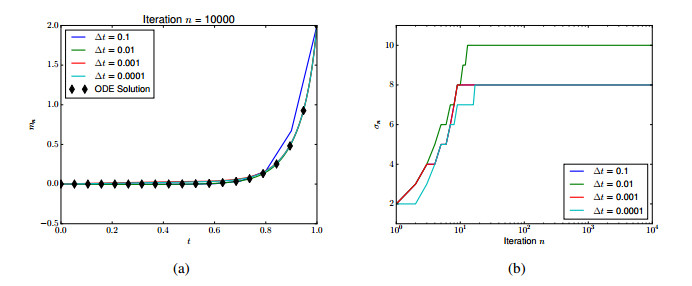
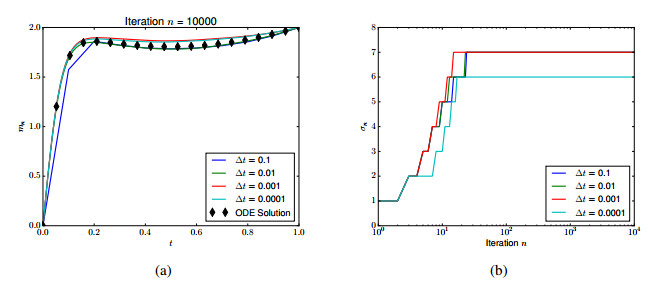
Since $\Phi''(v+m_0+\xi)\geq \epsilon^{-1}$, we are guaranteed convergence using expanding trust regions. Taking $\epsilon = 0.01$, $m_- = 0$ and $m_+ = 2$, this is illustrated in Figure 3, where we have also solved (4.8) by ODE methods for comparison. As trust regions, we take

and we always restart at the zero solution Figure 3 also shows robustness to discretization; the number of truncations is relatively insensitive to $\Delta t$.

4.4.   Locally convex example

For many problems of interest, we do not have global convexity. Consider the double well potential (4.3), but in the case of paths,

Then,

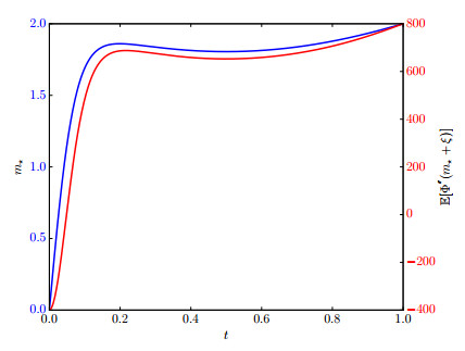
Here, we take $m_- = 0$, $m_+ = 2$, and $\epsilon = 0.01$. We have plotted the numerically solved ODE in Figure 4. Also plotted is $\mathbb{E}[\Phi''(v_\star +m_0+ \xi)]$. Note that $\mathbb{E}[\Phi''(v_\star +m_0+ \xi)]$ is not sign definite, becoming as small as $-400$. Since $C_0$ has $\lambda_1 = 1/\pi^2 \approx 0.101$, (3.15) cannot apply.

Discretizing the Schrödinger operator

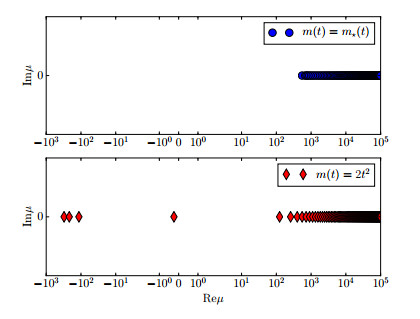
we numerically compute the eigenvalues. Plotted in Figure 5, we see that the minimal eigenvalue of $J''(m_\star)$ is approximately $\mu_1\approx 550$. Therefore,

for all $v$ in some neighborhood of $v_\star$. For an appropriately selected fixed trust region, the algorithm will converge.

However, we can show that the convexity condition is not global. Consider the path $m(t) = 2t^2$, which satisfies the boundary conditions. As shown in Figure 5, this path induces negative eigenvalues.

Despite this, we are still observe convergence. Using the fixed trust region

we obtain the results in Figure 6. Again, the convergence is robust to discretization.

5.   Discussion

We have shown that the Robbins-Monro algorithm, with both fixed and expanding trust regions, can be applied to Hilbert space valued problems, adapting the finite dimensional proof of ^[12]. We have also constructed sufficient conditions for which the relative entropy minimization problem fits within this framework.

One problem we did not address here was how to identify fixed trust regions. Indeed, that requires a tremendous amount of a priori information that is almost certainly not available. We interpret that result as a local convergence result that gives a theoretical basis for applying the algorithm. In practice, since the root is likely unknown, one might run some numerical experiments to identify a reasonable trust region, or just use expanding trust regions. The practitioner will find that the algorithm converges to a solution, though perhaps not the one originally envisioned. A more sophisticated analysis may address the convergence to a set of roots, while being agnostic as to which zero is found.

Another problem we did not address was how to optimize not just the mean, but also the covariance in the Gaussian. As discussed in ^[15], it is necessary to parameterize the covariance in some way, which will be application specific. Thus, while the form of the first variation of relative entropy with respect to the mean, (3.7), is quite generic, the corresponding expression for the covariance will be specific to the covariance parameterization. Additional constraints are also necessary to guarantee that the parameters always induce a covariance operator. We leave such specialization as future work.

Acknowledgments

This work was supported by US Department of Energy Award DE-SC0012733. This work was completed under US National Science Foundation Grant DMS-1818716. The authors would like to thank J. Lelong for helpful comments, along with anonymous reviewers whose reports significantly impacted our work.

Conflict of interest

The authors declare that there is no conflicts of interest in this paper.