Review Topical Sections

Smart materials for energy storage in Li-ion batteries

  • Advanced lithium-ion batteries contain smart materials having the function of insertion electrodes in the form of powders with specific and optimized electrochemical properties. Different classes can be considered: the surface modified active particles at either positive or negative electrodes, the nano-composite electrodes and the blended materials. In this paper, various systems are described, which illustrate the improvement of lithium-ion batteries in term of specific energy and power, thermal stability and life cycling.

    Citation: Christian M Julien, Alain Mauger, Ashraf E Abdel-Ghany, Ahmed M Hashem, Karim Zaghib. Smart materials for energy storage in Li-ion batteries[J]. AIMS Materials Science, 2016, 3(1): 137-148. doi: 10.3934/matersci.2016.1.137

    Related Papers:

    [1] Ying Li, Zhao Zhao, Yuan-yuan Tan, Xue Wang . Dynamical analysis of the effects of circadian clock on the neurotransmitter dopamine. Mathematical Biosciences and Engineering, 2023, 20(9): 16663-16677. doi: 10.3934/mbe.2023742
    [2] Jifa Jiang, Qiang Liu, Lei Niu . Theoretical investigation on models of circadian rhythms based on dimerization and proteolysis of PER and TIM. Mathematical Biosciences and Engineering, 2017, 14(5&6): 1247-1259. doi: 10.3934/mbe.2017064
    [3] Changgui Gu, Ping Wang, Tongfeng Weng, Huijie Yang, Jos Rohling . Heterogeneity of neuronal properties determines the collective behavior of the neurons in the suprachiasmatic nucleus. Mathematical Biosciences and Engineering, 2019, 16(4): 1893-1913. doi: 10.3934/mbe.2019092
    [4] E.V. Presnov, Z. Agur . The Role Of Time Delays, Slow Processes And Chaos In Modulating The Cell-Cycle Clock. Mathematical Biosciences and Engineering, 2005, 2(3): 625-642. doi: 10.3934/mbe.2005.2.625
    [5] Shishi Wang, Yuting Ding, Hongfan Lu, Silin Gong . Stability and bifurcation analysis of $ SIQR $ for the COVID-19 epidemic model with time delay. Mathematical Biosciences and Engineering, 2021, 18(5): 5505-5524. doi: 10.3934/mbe.2021278
    [6] Zhichao Jiang, Xiaohua Bi, Tongqian Zhang, B.G. Sampath Aruna Pradeep . Global Hopf bifurcation of a delayed phytoplankton-zooplankton system considering toxin producing effect and delay dependent coefficient. Mathematical Biosciences and Engineering, 2019, 16(5): 3807-3829. doi: 10.3934/mbe.2019188
    [7] Xin-You Meng, Yu-Qian Wu . Bifurcation analysis in a singular Beddington-DeAngelis predator-prey model with two delays and nonlinear predator harvesting. Mathematical Biosciences and Engineering, 2019, 16(4): 2668-2696. doi: 10.3934/mbe.2019133
    [8] Hongying Shu, Wanxiao Xu, Zenghui Hao . Global dynamics of an immunosuppressive infection model with stage structure. Mathematical Biosciences and Engineering, 2020, 17(3): 2082-2102. doi: 10.3934/mbe.2020111
    [9] Hongfan Lu, Yuting Ding, Silin Gong, Shishi Wang . Mathematical modeling and dynamic analysis of SIQR model with delay for pandemic COVID-19. Mathematical Biosciences and Engineering, 2021, 18(4): 3197-3214. doi: 10.3934/mbe.2021159
    [10] Xiaomeng Ma, Zhanbing Bai, Sujing Sun . Stability and bifurcation control for a fractional-order chemostat model with time delays and incommensurate orders. Mathematical Biosciences and Engineering, 2023, 20(1): 437-455. doi: 10.3934/mbe.2023020
  • Advanced lithium-ion batteries contain smart materials having the function of insertion electrodes in the form of powders with specific and optimized electrochemical properties. Different classes can be considered: the surface modified active particles at either positive or negative electrodes, the nano-composite electrodes and the blended materials. In this paper, various systems are described, which illustrate the improvement of lithium-ion batteries in term of specific energy and power, thermal stability and life cycling.


    1. Introduction

    Circadian clocks are endogenous 24-h oscillations that regulate the temporal organization of physiology, metabolism and behavior[4,11]. Disruption of circadian rhythms leads to various diseases and may reduce lifespan in mice [2,8,9,14]. The central mechanism of the mammalian circadian oscillation is a negative feedback loop that involves the transcriptional activator genes: clock and bmal1, and five repressor genes: period (per1-per3) and cryptochrome (cry1 and cry2)[11,20]. CLOCK and BMAL1 are transcription factors that activate per and cry gene transcriptions. The resulting PER and CRY proteins accumulate, and then inhibit CLOCK/BMAL1-mediated transcription after a certain time delay. Various auxiliary loops also take part in the regulation of mammalian circadian clocks. Previous studies validated that cry1 expression is positively auto-regulated via the inhibition of its repressor rev-erb$\alpha$, which forms a positive loop [16]. Some nuclear receptors, exhibiting circadian like patterns of expression [18], may also contribute to the circadian clock via other auxiliary loops. These auxiliary loops are believed to receive the environmental factors for adaption purpose, therefore provide multiple entry points to regulate the circadian oscillator. Therefore, an important question arises: How does the system with more than one feedback loop maintain the robustness of the oscillation?

    Goldbeter [5] proposed the first molecular model of circadian clock in Drosophila. This model takes account of the core negative feedback loop of per self-repression. Since then, a lot of mathematical models in different organisms based on the negative feedback loop have been developed and studied by many groups [6,10,15,19]. Recently, the circadian clock models with more than one feedback loops have been proposed, and the computational studies have revealed some interesting results [3,9,12,17]. However, the studies on the stability of the multi-loop regulation in circadian clock remain obscure.

    Here we consider a system of one differential equation modeling the transcriptional co-regulation in a mammalian circadian clock. In this system, there is a core feedback loop that CRY1 negatively regulates its own expression by inhibiting CLOCK/BMAL1-mediated transcription. A delay naturally appears in this process, representing the durations of post-translational regulations. There occurs another auxiliary loop in this model in which CRY1 positively mediates its own expression via the inhibition of its repressor rev-erb$\alpha$ (see Fig. 1). Similarly, this positive process also contains a time delay. Therefore, we consider a two-loop system with two time delays in this work. The theoretical approach is based on the work of Adimy et al.[1]. Our aim is to show that the auxiliary loops, which are linked to other pathways for adaption purpose, will not abandon the oscillation with reasonable parameters.

    Figure 1. The model of a mammalian circadian clock with two delays. Figure (a) is a schematic diagram of gene regulation in the mammalian circadian clock system, figure (b) is a schematic diagram of the simplified mathematical model of a mammalian circadian clock.

    This paper is organized as follows: Section 2 presents the model of a mammalian circadian clock, a scalar nonlinear delay differential equation with two delays, and investigates the existence of a nontrivial positive equilibrium point. Section 3 analyses the asymptotic stability of this equilibrium point. We first linearize the model about the equilibrium point and obtain a first degree exponential polynomial characteristic equation. Then we determine the conditions for the stability when only one delay is equal to zero, and, eventually, when both delays are nonzero. Besides, we also establish the existence of the Hopf bifurcations, which destabilizes the system and leads to the existence of periodic solutions. Section 4 numerically illustrates the theoretical results and Section 5 discusses the effect of time delays on the period of the model.


    2. The model

    In mammalian circadian clocks, there is a core negative feedback loop to drive the oscillation. CRY protein combines with PER to form the dimer CRY/PER, which translocates into nucleus to inhibit CLOCK/BMAL1-mediated transcription of cry1, see Fig. 1(a). Besides the core loop, there are also some auxiliary loops in the mammalian circadian system to co-regulate clock. In this work, we focus on an important auxiliary loop via rev-erb$\alpha$. The transcription of rev-erb$\alpha$ is also mediated by CLOCK/BMAL1 complex, so that can be inhibited by CRY/PER complex. In return, REV-ERB$\alpha$ feeds back to repress the transcription of cry1. The double-inhibition process forms a positive feedback loop (see Fig. 1(a)).

    Our previous work about this system [17] illustrated some interesting numerical results. In order to obtain the theoretical insights of it, we first reduce the variables to form a simple one-dimensional system. We denote by $x(t)$ the mRNA concentration of cry1 at time $t$. The transcription rate of cry1 (the synthesis rate of $x(t)$) is regulated by two items: one is the negative feedback through CLOCK/BMAL1 complex after a time delay $\tau_1$, and the other one is the positive feedback through REV-ERB$\alpha$ after a time delay $\tau_2$ (see Fig. 1(b)). The degradation rate of cry1 mRNA is simply assumed to be proportional to itself. Therefore, the equation modeling the co-regulation of multiple loops in mammalian circadian clocks is:

    $\frac{dx}{dt}=\frac{k_1}{M+x^2(t-\tau_1)}+k_2x(t-\tau_2)-cx(t),$ (2.1)

    where $k_1$ and $M$ are positive constants describing the negative regulation, $k_2$ is a positive constant characterizing the strength of positive regulation, and the constant $c >0$ reflects the linear degradation rate. The parameter $\tau_1 > 0$ denotes the average time needed by the negative feedback, which represents the durations of post-translational regulations. The parameter $\tau_2 > 0$ denotes the average time needed by the positive feedback.

    Obviously, system (2.1) has a unique continuous solution $x(t)$ which is well-defined for all $t\geq0$ and for a continuous initial condition. Furthermore, it is easy to see that, for nonnegative initial conditions, the solutions of (2.1) remain nonnegative for $t\geq0$. In fact, if we let $t_0 > 0$ be such that $x(t)> 0$ for $t < t_0$ and $x(t_0) = 0, $ then, from (2.1), we have

    $\frac{dx(t_0)}{dt}=\frac{k_1}{M+x^2(t_0-\tau_1)}+k_2x(t_0-\tau_2)>0, $

    and the result follows.

    Now, we begin to consider the existence of equilibrium points for system (2.1). An equilibrium point of system (2.1) is a stationary solution $x^{\ast}$ of (2.1), that is,

    $ (k_2-c)(x^{\ast})^3+M(k_2-c)x^{\ast}+k_1=0.$ (2.2)

    Evidently, $0$ is not an equilibrium point of system (2.1), so it is enough to search for its nonzero equilibrium points. For this purpose, we need to assume that $c>k_2$ and recall the well-known Shengjin's formulas.

    Lemma 2.1. (Shengjin's formulas) Consider a variable cubic equationt

    $ ax^3+bx^2+cx+d=0, $ (2.3)

    where $ a, b, c, d \in R, \mbox{and}\ a\neq 0.$ Set repeated root discriminant $ A=b^2-3ac, \ B=bc-9ad, \ C=c^2-3bd, $ and total discriminant $ \Delta=B^2-4AC.$ Then the following statements are true:

    ( $i$ ) When $A=B=0, $ (2.3) has a triple real root $x_1=x_2=x_3=-\frac{b}{3a}=-\frac{c}{b} =-\frac{3d}{c};$

    ( $ii$ ) When $ \Delta=B^2-4AC >0, $ (2.3) has a real root $ x^{\ast}=\frac{-b-(\sqrt[3]{Y_1}+\sqrt[3]{Y_2})}{3a}$ and a pair of conjugate complex roots, where $ Y_{1, 2}=Ab+3a\left( \frac{-B\pm\sqrt{B^2-4AC}}{2}\right)$;

    ( $iii$ ) When $\Delta=B^2-4AC =0, $ (2.3) has three real roots $x_1=-\frac{b}{a}+K, \ x_2=x_3=-\frac{K}{2}, $ where $K=\frac{B}{A}, \, A\neq 0;$

    ( $iv$ ) When $\Delta=B^2-4AC <0, $ (2.3) has three unequal real roots.

    Using Lemma 2.1, in Eq.(2.2), we calculate

    $ A=-3M(k_2-c)^2, B=-9k_1(k_2-c), C=M^2(k_2-c)^2, $

    and obtain

    $ \Delta =B^2-4AC=(k_2-c)^2\left(81k_1^2+12M^3(k_2-d)^2\right)>0, $

    then it follows from Lemma 2.1 (ii) that Eq.(2.2) has a real root $x=x^{\ast}=\frac{\sqrt[3]{Y_1}+\sqrt[3]{Y_2}}{3(c-k_2)}, $ where

    $Y_1=\frac{3}{2}(k_2-c)^2\left( 9k_1+\sqrt{81k_1^2+12M^3(k_2-c)^2}\right), $
    $ Y_2=\frac{3}{2}(k_2-c)^2\left( 9k_1-\sqrt{81k_1^2+12M^3(k_2-c)^2}\right). $

    In addition, we can easily see that $Y_1+Y_2=27k_1(k_2-c)^2>0, $ leading to $Y_1>-Y_2$ and $\sqrt[3]{Y_1} > -\sqrt[3]{Y_2}, $ which implies $\sqrt[3]{Y_1} +\sqrt[3]{Y_2} >0. $ Consequently, Eq. (2.2) has a positive solution, which is unique if and only if $c>k_2.$

    This result is summarized in the following proposition.

    Proposition 2.1. Assume that $c>k_2.$ Then system (2.1) has a unique nontrivial positive equilibrium point $x^{\ast}$, a solution of Eq.(2.2).


    3. Local asymptotic stability

    In this section, we concentrate on the stability of the nontrivial equilibrium point $x^{\ast}$. Hence, we assume throughout this section that $c>k_2.$

    We first start to linearize system (2.1) around $x^{\ast}$ and deduce the characteristic equation.


    3.1. Linearization and characteristic equation

    Take $y(t)=x(t)-x^{\ast}, $ the linearized system of (2.1) about $x^{\ast}$ is then given by

    $\frac{dy}{dt}=-\frac{2k_1x^{\ast}}{(M+x^{\ast^2})^2}y(t-\tau_1)+k_2y(t-\tau_2)-cy(t), $ (3.1)

    Denote

    $\alpha=\frac{2k_1x^{\ast}}{(M+x^{\ast^2})^2}, \beta=k_2.$ (3.2)

    The characteristic equation associated with (3.1) is given by

    $\lambda +\alpha e^{-\lambda\tau_1}-\beta e^{-\lambda\tau_2}+c=0.$ (3.3)

    Through studying the sign of the real parts of roots of (3.3), we can analyse the local asymptotic stability of the equilibrium point $x^{\ast}$. Here we recall that $x^{\ast}$ is locally asymptotically stable if and only if all roots of (3.3) have negative real parts, and its stability can only be lost if roots cross the vertical axis, that is, if purely imaginary roots appear.

    Because of the presence of two different delays, $\tau_1$ and $\tau_2$, in Eq.(3.3), it is very complicated to analyse the sign of the real parts of eigenvalues, and there is no direct approaches to be considered. In the following, on the base of the analytic methods as in Ruan and Wei [13], we will discuss the stability of the equilibrium point when one delay is equal to zero, and deduce conditions for the stability of the equilibrium point when both time delays are nonzero.


    3.2. The case $\tau_1=\tau_2=0$

    Assume that $\tau_1=\tau_2=0$. Then, the characteristic Eq.(3.3) is written as a first degree polynomial equation

    $ \lambda+\alpha-\beta+c=0.$ (3.4)

    Obviously, the only eigenvalue of (3.4) is $\lambda=-\alpha+\beta-c.$ It is seen that $\lambda <0$ because of the assumption $ c >\beta=k_2.$ We can then conclude the asymptotic stability of $x^{\ast}$ when $\tau_1=\tau_2=0$ in the next proposition.

    Proposition 3.1. Assume that $ c >\beta.$ Then all eigenvalues of (3.3) have negative real parts, and the equilibrium point $x^{\ast}$ of system (2.1) is locally asymptotically stable.


    3.3. The case $\tau_1>0, \ \tau_2=0$

    We now consider the case $\tau_1>0$ and $\tau_2=0.$ Setting $\tau_2=0$ in (3.3), the characteristic equation becomes

    $\lambda +\alpha e^{-\lambda\tau_1}-\beta+c=0.$ (3.5)

    When $\tau_1$ increases, the stability of the equilibrium point $x^{\ast}$ can be lost only if pure imaginary roots appear. Hence we look for purely imaginary roots $ \lambda=\pm i\omega, \, \omega \in \mathbb{R}$, of (3.5).

    If $i\omega$ is a purely imaginary root of (3.5), then separating real and imaginary parts, $\omega$ satisfies

    $\alpha\cos(\omega\tau_1)=\beta-c, \alpha\sin(\omega\tau_1)=\omega.$ (3.6)

    One can notice that if $\omega$ is a solution of (3.6), then so is $-\omega$. Thus, in the following, we only look for positive solutions $\omega$ of (3.6).

    Adding the squares of both hand sides of Eq.(3.6), we see that $\omega$ must be a root of the following equation:

    $\omega^2-\alpha^2+(c-\beta)^2=0.$ (3.7)

    Set $F(X)= X^2-\alpha^2+(c-\beta)^2$ and make the two assumptions as follows

    $ \mathrm{(H1)}\ \alpha \leq c-\beta;$

    $\mbox{(H2)}\ \alpha > c-\beta.$

    The function $F$ has no positive zeros when (H1) holds. When (H2) holds, the function $F$ has a unique positive zero $ \omega_0=\sqrt{\alpha^2-(c-\beta)^2}.$ Substituting $ \omega_0$ into Eq.(3.6), we have

    $ \tau_1^k=\frac{1}{\omega_0}\left( \arctan\left( \frac{\omega_0}{\beta-c}\right)+(2k+1)\pi\right), \ k=0, 1, 2, \cdots.$ (3.8)

    In addition, by differentiating (3.5) with respect to $\tau_1$, we obtain

    $ (1-\alpha\tau_1e^{-\lambda\tau_1})\frac{d\lambda}{d\tau_1}-\alpha\lambda e^{-\lambda\tau_1}=0.$ (3.9)

    From (3.9), we deduce that

    $ \left(\frac{d\lambda}{d\tau_1}\right)^{-1}=\frac{1-\alpha\tau_1e^{-\lambda\tau_1}}{\alpha\lambda e^{-\lambda\tau_1}}=\frac{e^{\lambda\tau_1}}{\alpha\lambda}-\frac{\tau_1}{\lambda}.$

    Then,

    $ \mathrm{Re}\left(\frac{d\lambda}{d\tau_1}\right)^{-1}_{\lambda=i\omega_0} = \mathrm{Re}\left(\frac{e^{\lambda\tau_1}}{\alpha\lambda}-\frac{\tau_1}{\lambda}\right)_{\lambda=i\omega_0}=\frac{1}{\omega_0\alpha}\sin(\omega_0\tau_1).$

    Combining with (3.6), we get

    $ \mathrm{Re}\left(\frac{d\lambda}{d\tau_1}\right)^{-1}_{\lambda=i\omega_0}= \frac{1}{\alpha^2}>0, $

    which means

    $ \frac{d\mathrm{Re}(\lambda)}{d\tau_1}\mid_{\lambda=i\omega_0}=\mathrm{Re}\left(\frac{d\lambda}{d\tau_1}\right)_{\lambda=i\omega_0} >0.$

    Based on the above analysis, we obtain the following Lemma 3.1.

    Lemma 3.1. Let $\tau_1^k$ be defined by (3.8).

    ( $i$ ) If (H1) holds, the characteristic Eq.(3.5) has no imaginary roots;

    ( $ii$ ) If (H2) holds, for $\tau_1=\tau_1^k, $ the characteristic Eq.(3.5) has a pair of simple conjugate pure imaginary roots $ \pm i\omega_0$, satisfying

    $ \frac{d \mathrm{Re}(\lambda)}{d\tau_1}\mid_{\lambda=i\omega_0} >0.$

    According to Lemma 3.1 and the Hopf bifurcation theorem for delay differential equations, we conclude, the stability of the equilibrium point $x^{\ast}$ of (2.1) when $\tau_1>0, \ \tau_2=0, $ in the following theorem.

    Theorem 3.1. Assume that $(H2)$ holds and $\tau_2=0$. Let $\tau_1^0$ be defined by (3.8). Then

    ( $i$ ) when $\tau_1\in(0, \tau_1^0)$, the positive equilibrium point $x^{\ast}$ of system (2.1) is locally asymptotically stable;

    ( $ii$ ) there exists an enough small number $\epsilon>0 $ such that the positive equilibrium point $x^{\ast}$ of system (2.1) is unstable when $\tau_1\in(\tau_1^0, \, \tau_1^0+\epsilon)$;

    ( $iii$ ) when $\tau_1= \tau_1^0, $ a Hopf bifurcation occurs at the positive equilibrium point $x^{\ast}$ of system (2.1).


    3.4. The case $\tau_1>0, \ \tau_2> 0$

    We now return to investigate Eq.(3.3) with $\tau_1>0, \ \tau_2> 0$. In order to study the local stability of the equilibrium point $x^{\ast}$ of (2.1), we regard $\tau_2$ as a bifurcation parameter, take $\tau_1=\tau_1^{\ast}\in(0, \infty), $ and discuss the distribution of the roots of the following characteristic equation

    $\lambda +\alpha e^{-\lambda\tau_1^{\ast}}-\beta e^{-\lambda\tau_2}+c=0.$ (3.10)

    We first verified a result concerning the sign of the real parts of characteristic roots of (3.10) with $\tau_1^{\ast}\in(0, \tau_1^0)$ in the following lemma.

    Lemma 3.2. If all roots of Eq.(3.5) have negative real parts for $\tau_1^{\ast}\in(0, \tau_1^0), $ then there exists a $\tau_2^{\ast}(\tau_1^{\ast})>0$ such that all roots of Eq.(3.10) have negative real parts when $\tau_2<\tau_2^{\ast}(\tau_1^{\ast}).$

    Proof. From Theorem 3.1 (ⅰ), we know that Eq.(3.5) has no root with nonnegative real part for $\tau_1^{\ast}\in(0, \tau_1^0).$ Obviously, the left hand side of Eq.(3.10) is analytic in $\lambda$ and $\tau_2$. Following Theorem 2.1 of Ruan and Wei [13], as the parameter $\tau_2$ varies, the sum of the multiplicity of zeros of the left hand side of Eq.(3.3) in the open right half-plane can change only if a zero appears on or crosses the imaginary axis.

    Since Eq.(3.10) with $\tau_2=0 $ has no root with nonnegative real part when $\tau_1^{\ast}\in(0, \tau_1^0), $ there exists a $\tau_2^{\ast}(\tau_1^{\ast})$ such that all roots of Eq.(3.10) have negative real parts when $\tau_2<\tau_2^{\ast}(\tau_1^{\ast})$.

    Lemma 3.3. If $\tau_1^{\ast}\in(\tau_1^0, \, \tau_1^0+\epsilon), $ then there exists a positive number $\tau_2^{\ast\ast}(\tau_1^{\ast})$ such that Eq.(3.10) has at least one root with strictly positive real parts when $\tau_2<\tau_2^{\ast\ast}(\tau_1^{\ast}).$

    Proof. Let $\lambda$ be a zero of the left hand side of Eq.(3.10) satisfying $\mathrm{Re}\lambda\geq0.$ Then from (3.10), we can obtain

    $ \lambda =-\alpha e^{-\lambda\tau_1^{\ast}}+\beta e^{-\lambda\tau_2}-c, $

    and

    $ |\lambda|\leq \alpha e^{-\lambda\tau_1^{\ast}}+\beta e^{-\lambda\tau_2}+c\leq \alpha + \beta+c, $

    which shows that the zeros of the left hand side of Eq.(3.10) in the open right half plane are uniformly bounded. Furthermore, the left hand side of Eq.(3.10) is an elementary analytic function with regard to $\lambda$ and $\tau_2$. Therefore, according to Corollary 2.4 in Ruan and Wei [13], as the parameter $\tau_2$ varies, the sum of the multiplicity of zeros of the left hand side of Eq.(3.3) in the open right half-plane can only change if a zero appears on or crosses the imaginary axis.

    Since Eq.(3.5) has at least one root with strictly positive real parts when $\tau_1^{\ast}\in(\tau_1^0, \tau_1^0+\epsilon)$ with $\epsilon>0, $ the left hand side of Eq.(3.10) with $\tau_2=0 $ has no zeros appearing on the imaginary axis by Lemma 3.1 (ii). Thus, there must exist a positive number $\tau_2^{\ast\ast}(\tau_1^{\ast})$ such that the sum of the orders of the zeros of the left hand side of Eq.(3.10) in the open right half plane is a fixed number when $\tau_2<\tau_2^{\ast\ast}(\tau_1^{\ast})$, which means that Eq.(3.10) has at least one root with strictly positive real parts when $\tau_2<\tau_2^{\ast\ast}(\tau_1^{\ast})$.

    From Lemmas 3.2 and 3.3, we have the following theorem concerning the stability of the equilibrium point $x^{\ast}$ of (2.1) when $\tau_1>0, \ \tau_2> 0$.

    Theorem 3.2. Let $ \tau_1=\tau_1^{\ast}\in(0, \infty), \ \tau_2\in(0, \infty).$

    ( $i$ ) If $\tau_1^{\ast}\in(0, \tau_1^0), $ then there exists a number $\tau_2^{\ast}(\tau_1^{\ast})>0$ such that the positive equilibrium point $x^{\ast}$ of system (2.1) is locally asymptotically stable when $\tau_2<\tau_2^{\ast}(\tau_1^{\ast}).$

    ( $ii$ ) If $\tau_1^{\ast}\in(\tau_1^0, \tau_1^0+\epsilon)$ with $\epsilon>0$, then there exists a number $\tau_2^{\ast\ast}(\tau_1^{\ast})>0$ such that the positive equilibrium point $x^{\ast}$ of system (2.1) is unstable when $\tau_2<\tau_2^{\ast\ast}(\tau_1^{\ast}).$

    Proof. First we let $\tau_1^{\ast}\in(0, \tau_1^0).$ Then from Lemma 3.2, there exists a $\tau_2^{\ast}(\tau_1^{\ast})>0$ such that all roots of Eq.(3.10) have negative real parts when $\tau_2<\tau_2^{\ast}(\tau_1^{\ast}), $ which shows that (ⅰ) follows.

    Secondly, we let $\tau_1^{\ast}\in(\tau_1^0, \tau_1^0+\epsilon)$ with $\epsilon>0.$ Then according to Lemma 3.3, that there exists a positive number $\tau_2^{\ast\ast}(\tau_1^{\ast})$ such that Eq.(3.10) has at least one root with strictly positive real parts when $\tau_2<\tau_2^{\ast\ast}(\tau_1^{\ast})$, which means that statement (ⅱ) is true.

    Next, we look for purely imaginary roots $ \lambda= \pm iv$ of Eq.(3.10) for $ \tau_1^{\ast}\in(0, \infty)$, where $ v=v(\tau_2)>0$. Substituting $\lambda= iv$ into (3.10), we have

    $iv+\alpha(\cos(v\tau_1^{\ast})-i\sin(v\tau_1^{\ast}))-\beta(\cos(v\tau_2)-i\sin(v\tau_2))+c=0, $

    then separating real and imaginary parts in the above equality, $v$ satisfies

    $\beta\cos(v\tau_2)=\alpha\cos(v\tau_1^{\ast})+c, \beta\sin(v\tau_2)=\alpha\sin(v\tau_1^{\ast})-v.$ (3.11)

    Adding the squares to both sides of each equation in (3.10), we see that $v$ must be a root of the following equation:

    $ v^2+2c\alpha\cos(v\tau_1^{\ast})-2\alpha v \sin(v\tau_1^{\ast})+\alpha^2+c^2-\beta^2=0. $ (3.12)

    Let

    $f(v)=v^2+\alpha^2+c^2-\beta^2, g(v)=-2c\alpha\cos(v\tau_1^{\ast})+2\alpha v \sin(v\tau_1^{\ast}).$ (3.13)

    Then Eq.(3.12) is equivalent to the following equation

    $f(v)= g(v).$ (3.14)

    Now, we establish the sufficient conditions for the existence of positive solutions of Eq.(3.14) as follows.

    Proposition 3.2. If there exists a positive number $\tilde{v}$ satisfying

    $ f(\tilde{v})< g(\tilde{v}),$ (3.15)

    then there exists at least one positive number $v_0 \in (0, \, \tilde{v})$ such that $f(v_0)=g(v_0)$.

    Proof. Let $F(v)=f(v)-g(v).$ Obviously, $F(v)$ is continuous on the interval [0, $\tilde{v}$]. From (3.13) and (3.15), we see $ F(0)>0, \ F(\tilde{v})<0.$ Then the conclusion is true according to intermediate value theorem.

    If the condition of Proposition 3.2 holds, then Eq.(3.12) has at least one positive solution $v_0$. Thus we obtain from (3.11)

    $\tau_{2}^j =\\ \left\{
    1v0(arctan(αsin(v0τ1)v0αcos(v0τ1)+c)+2jπ), j=0,1,, if v0τ2j lies in the first quadrant;(2j+12)πv0, j=0,1,,if v0τ2j appears on the upper half imaginary axis;1v0(arctan(αsin(v0τ1)v0αcos(v0τ1)+c)+π+2jπ), j=0,1,, if v0τ2j lies in the second quadrant;(2j+1)πv0, j=0,1,,if v0τ2j appears on the negative real axis;1v0(arctan(αsin(v0τ1)v0αcos(v0τ1)+c)π+2jπ), j=1,2,, if v0τ2j lies in the third quadrant;(2j12)πv0, j=1,2,,if v0τ2j appears on the lower half imaginary axis;1v0(arctan(αsin(v0τ1)v0αcos(v0τ1)+c)+2jπ), j=1,2,,if v0τ2j lies in the fourth quadrant;2jπv0, j=1,2,,if v0τ2j appears on the positive real axis.
    \right.$
    (3.16)

    Based on the above analysis, we obtain the following theorem.

    Theorem 3.3. Let $\tau_{2}^j, \ j=0, 1, 2, \ldots$ be defined by (3.16). For $\tau_1=\tau_1^{\ast}\in(0, \, \infty), \, \tau_2 =\tau_{2}^j, \ j=0, 1, 2, \ldots, $ the characteristic Eq.(3.3) has a pair of simple conjugate purely imaginary roots $\pm i v_0$ satisfying

    $\mathrm{sign}\left\{\frac{d \mathrm{Re}\lambda}{d\tau_2}|_{\lambda=iv_0}\right\}=\mathrm{sign}(g(v_0, \tau_1^{\ast})), $

    where

    $ g(v_0, \tau_1^{\ast})=v_0(1-\alpha\tau_1^{\ast}\cos(v_0\tau_1^{\ast}))-(1+\tau_1^{\ast}c)\alpha\sin(v_0\tau_1^{\ast})\neq 0.$ (3.17)

    Proof. It is easy to see from (3.11)-(3.14) that the characteristic Eq.(3.7) has a pair of simple conjugate pure imaginary roots $\pm i v_0.$ Further, by differentiating (3.10) with respect to $\tau_2$, we deduce that

    $ \left(\frac{d\lambda}{d\tau_2}\right)^{-1}=-\frac{e^{\lambda\tau_2}}{\lambda\beta}+\frac{\alpha\tau_1^{\ast}}{\lambda\beta}e^{-\lambda(\tau_1^{\ast}-\tau_2)}-\frac{\tau_2}{\lambda}.$

    Then

    $\mathrm{ Re}\left(\frac{d\lambda}{d\tau_2}\right)^{-1}_{\lambda=iv_0}=-\frac{\alpha\tau_1^{\ast}}{v_0\beta}\sin(v_0\tau_1^{\ast})\cos(v_0\tau_2) +\left(\frac{\alpha\tau_1^{\ast}}{v_0\beta}\cos(v_0\tau_1^{\ast}) -\frac{1}{v_0\beta}\right)\sin(v_0\tau_2). $

    Combining with (3.12), we simplify the above equality and obtain

    $\mathrm{ Re}\left(\frac{d\lambda}{d\tau_2}\right)^{-1}_{\lambda=iv_0} =\frac{1}{v_0\beta^2}\left[v_0(1-\alpha\tau_1^{\ast}\cos(v_0\tau_1^{\ast}))-(1+\tau_1^{\ast}c)\alpha\sin(v_0\tau_1^{\ast})\right]=\frac{1}{v_0\beta^2}g(v_0, \tau_1^{\ast}). $

    Based on (3.17) and (3.18), we conclude that

    $\mathrm{sign}\left\{\frac{d \mathrm{Re}\lambda}{d\tau_2}|_{\lambda=iv_0}\right\}=\mathrm{sign}\left\{\mathrm{ Re}\left(\frac{d\lambda}{d\tau_2}\right)^{-1}_{\lambda=iv_0}\right\}=\mathrm{sign}(g(v_0, \tau_1^{\ast})).$

    Remark 3.1. From Theorem 3.3, it is followed that $\frac{d \mathrm{Re}\lambda}{d\tau_2}\mid_{\lambda=iv_0}> 0$ if $g(v_0, \tau_1^{\ast})>0, $ and $\frac{d \mathrm{Re}\lambda}{d\tau_2}\mid_{\lambda=iv_0}< 0$ if $g(v_0, \tau_1^{\ast})<0.$

    Remark 3.2. We can also make similar discussions if we let $\tau_1=0, $ and regard $\tau_2$ as a parameter.


    4. Numerical simulations

    In this section, we illustrate the different stability results obtained in the previous sections, mainly in Theorems 3.1 and 3.2. We also focus on periodic solutions appearing through a Hopf bifurcation. Without loss of generality, we take time unit as an hour, and let initial condition be $x_0=0.1.$

    Assuming $k_1=4.5, \ k_2=0.15, \ c=1, \ M=0.5, $ then system (2.1) becomes

    $\frac{dx}{dt}=\frac{4.5}{0.5+x^2(t-\tau_1)}+0.15x(t-\tau_2)-x.$ (4.1)

    Firstly, we illustrate the stability and Hopf bifurcation of the equilibrium of system (4.1) when $\tau_1>0, \ \tau_2=0.$ In this case, system (4.1) is reduced to

    $\frac{dx}{dt}=\frac{4.5}{0.5+x^2(t-\tau_1)}-0.85x.$ (4.2)

    From (4.2), we get a positive equilibrium point $x^{\ast}=1.6473.$ From (3.2), we calculate $\alpha= 1.4355, \ c-\beta=0.85, $ satisfying (H2). Based on (3.8), we have $\omega_0=\sqrt{\alpha^2-(c-\beta)^2}=1.1568, \ \tau_1^0=1.9057.$ Then according to Theorem 3.1 we see that the equilibrium point $x^{\ast}=1.6473$ of system (4.2) is locally asymptotically stable when $\tau_1\in(0, \tau_1^0).$ When $\tau_1$ is gradually increasing and exceeds the critical value $\tau_1^{\ast}=\tau_1^0=1.9057, $ system (4.2) changes from stability to instability at the positive equilibrium point and thus a Hopf bifurcation occurs. Then we stimulate the change of system (4.2) when $\tau_1=0.5, \ \tau_1=1.5$ and $\tau_1=2.0, \ \tau_1=4.0$ respectively, and find the simulation results are in accordance with Theorem 3.1 (see Fig. 2).

    Figure 2. Stability and Hopf bifurcation of system (4.1) for different $\tau_1\in [0, \, \infty)$ when $\tau_2=0$. The equilibrium point $x^{\ast}$ of (4.2) is locally asymptotically stable when $\tau_1=0.5$ in figure (a) and $ \tau_1=1.5$ in figure (b), respectively. The equilibrium point $x^{\ast}$ of (4.2) losts its stability and stable bifurcation periodic solutions appear when $\tau_1=2.0$ in figure (c) and $ \tau_1=4.0$ in figure (d), respectively.

    Secondly, we illustrate the stability and Hopf bifurcation of the equilibrium of system (4.1) according to Theorem 3.2 when $ \tau_1>0, \ \tau_2>0$. Now we take $\tau_1^{\ast}=1.85 \in (0, \tau_1^0).$ Then according to Theorem 3.2 (i) and (3.16), we can find a critical value $\tau_2^{\ast}(\tau_1^{\ast})=4.05$ such that the equilibrium point $x^{\ast}$ of (4.1) is locally asymptotically stable when $0<\tau_2 < 4.05$. We simulate the change of system (4.1) when $0<\tau_2 < 4.05$ and find the simulation results are in accordance with the theoretical analysis results when $\tau_2=0.5, \ \tau_2=1.5, \ \tau_2=3.5, \ \tau_2=4$, respectively (see Fig. 3).

    Figure 3. Stability of system (4.1) with different $\tau_2$ when $\tau_1^{\ast}=1.85 \in (0, \tau_1^0)$ and $0<\tau_2 < 4.05$. The equilibrium point $x^{\ast}$ of (4.1) is locally asymptotically stable when $\tau_2=0.5$ in figure (a), $\tau_2=1.5$ in figure (b), $\tau_2=3.5$ in figure (c), $\tau_2=4$ in figure (d), respectively.

    Next, we take $\tau_1^{\ast}=2.8 \in (\tau_1^0, \infty)$. According to Theorem 3.2 (ii) and (3.16), we can find a critical value $\tau_2^{\ast}(\tau_1^{\ast})=2.1$ such that the equilibrium point $x^{\ast}$ of (4.1) is unstable when $0<\tau_2 < 2.1$. Then we simulate the change of system (4.1) when $0<\tau_2 < 2.1$ and find the simulation results correspond to the theoretical analysis results when $\tau_2=0.5, \ \tau_2=1, \ \tau_2=1.5, \ \tau_2=2$, respectively (see Fig. 4).

    Figure 4. Instability of system (4.1) with different $\tau_2$ when $\tau_1^{\ast}=2.8 \in (\tau_1^0, \infty)$ and $0<\tau_2 < 2.1$. The equilibrium point $x^{\ast}$ of (4.1) is unstable when $\tau_2=0.5$ in figure (a), $\tau_2=1$ in figure (b), $\tau_2=1.5$ in figure (c), $\tau_2=2$ in figure (d), respectively.

    From Fig. 3 and Fig. 4, it is seen that we just fix $\tau_1^{\ast}=1.85$ or $\tau_1^{\ast}=2.8$, and consider $\tau_2$ impacting on the stability of system (4.1). In fact, based on (3.16), we can obtain a series of corresponding critical value of $\tau_2$ for every given $\tau_1^{\ast}$. Thus, we have the bifurcation diagram of the parameters $\tau_1$ and $\tau_2$ (see Fig. 5).

    Figure 5. Bifurcation diagram of ($\tau_1, \, \tau_2$) for system (4.1). $S$ denotes stable regions, $US$ denotes oscillating regions. The black solid line is made up of critical bifurcation points for ($\tau_1, \, \tau_2$), the rest solid lines with different colours are lines consisting of critical bifurcation points when $\tau_2$ pluses different period respectively, and the marked six different points represent different values of ($\tau_1, \, \tau_2$).

    From Fig. 5, we can see that system (4.1) turns its instability into stability, or turns its stability into instability on both sides of the bifurcation line. Especially, when we fix $\tau_1=2.4$ and take $ \tau_2=0.5, \ 2, \ 5, \ 9, \ 12, \ 15.5$ which correspond to the six different points in Fig. 5, we simulate the stability of system 4.1 (see Fig. 6).

    Figure 6. Stability of system (4.1) with different $\tau_2$ when $\tau_1^{\ast}=2.4\in (\tau_1^0, \infty)$ and $\tau_2>0$. The equilibrium point $x^{\ast}$ of (4.1) is locally asymptotically stable when $\tau_2=2$ in figure (b), $\tau_2=9$ in figure (d), $\tau_2=15.5$ in figure (f), respectively, it is unstable when $\tau_2=0.5$ in figure (a), $\tau_2=5$ in figure (c), $\tau_2=12$ in figure (e), respectively.

    Furthermore, in order to verify the theoretical result of the bifurcation Fig. 5, we use numerical simulations and obtain all the values of $\tau_1, \, \tau_2$ which make system (4.1) generate oscillations (see Fig. 7).

    Figure 7. Oscillating range of ($\tau_1, \, \tau_2$) for system (4.1). Black regions represent oscillating solutions with periods for system (4.1) when ($\tau_1, \, \tau_2$) locates in the black region.

    From Fig. 7, we can see that the equilibrium point $x^{\ast}$ of system (4.1) is unstable when ($\tau_1, \, \tau_2$) locates in the black region, that is to say, system (4.1) generates oscillating solutions. The oscillating range of ($\tau_1, \, \tau_2$) is in accordance with the result of theoretical calculations in Fig. 5.


    5. Discussion

    In the previous researched circadian clock models with a time delay, it is found that the period of the model monotonously increases with the increase of the delay. In this paper, there are two different delays in our discussing biological clock model. To analyse the characteristic equation with two delays, we first concentrated on the case when one of the delays, $\tau_2$ equals zero and obtained a critical value for the delay $\tau_1$ : when $\tau_1<\tau_1^0 $ all roots of the characteristic equation have negative parts and when $\tau_1=\tau_1^0 $ purely imaginary roots appear. Then we assumed that $\tau_1=\tau_1^{\ast}<\tau_1^0 $ and considered the delay $\tau_2$ as a parameter. It showed that there exists a $ \tau_2^{\ast}(\tau_1^{\ast})$ such that all roots of the characteristic equation have negative real parts when $\tau_2\in (0, \tau_2^{\ast}(\tau_1^{\ast}))$. Finally, we assumed that $\tau_1=\tau_1^{\ast}\in(\tau_1^0, \, \tau_1^0+\epsilon)$ with $\epsilon >0$ and considered the delay $\tau_2$ as a parameter. We concluded that there exists a $ \tau_2^{\ast\ast}(\tau_1^{\ast})$ such that the characteristic equation has at least one root with strictly positive real parts when $\tau_2\in (0, \tau_2^{\ast\ast}(\tau_1^{\ast}))$. Consequently, we obtained stability and instability results for the mammalian circadian clock model with two independent delays respectively. The numerical results in Fig. 5 also indicate the existence of a Hopf bifurcation that leads to the emergence of periodic solutions.

    When discussing a mammalian circadian clock model with two delays, we found delays can affect the period of the model. When we first fix $\tau_2=29, $ assuming that $\tau_{1}$ ranges from $0$ to $12$, then fix $\tau_1=10, $ assuming that $\tau_{2}$ ranges from $0$ to $35, $ we numerically simulated the influence of delays on the period of model (4.1)(see Fig. 8).

    Figure 8. The effect of time delays on the period of system (4.1). In figure (a), we fix $\tau_2=29, $ the black solid line represents the relation between $\tau_1$ and the period. In figure (b), we fix $\tau_1=10, $ the black solid line represents $\tau_2$ and the period.

    From Fig. 8(a), we can see the period is monotonously increasing with the increase of time delay $\tau_1$ when $\tau_2=29$, which is in accord with that of a biological clock model with a single delay. However, from Fig. 8(b), we find that the period emerges non-monotonic regular variety with the increase of time delay $\tau_2$ when $\tau_1=10.$

    All in all, it is seen from Fig. 8 that $\tau_1$ determines the length of time. When $\tau_1$ is fixed, $\tau_2$ is changed, the period can only change in a certain range, which shows that the positive feedback between CRY1 and REV-ERB$\alpha$ in mammalian circadian clocks can benefit the robustness of the period length.


    Acknowledgments

    We would like to thank the reviewers and the editor for their valuable suggestions.


    [1] https://en.wikipedia.org/wiki/Smart_material (2015)
    [2] Julien CM, Mauger A, Vijh A, et al. (2015) Lithium Batteries: Science and Technology. Springer, New York.
    [3] Julien CM (2003) Lithium intercalated compounds, charge transfer and related properties. Mater Sci Eng R 40: 47–102. doi: 10.1016/S0927-796X(02)00104-3
    [4] Mauger A, Julien CM (2014) Surface modifications of electrode materials for lithium-ion batteries: status and trends. Ionics 20: 751–787. doi: 10.1007/s11581-014-1131-2
    [5] Hashem AMA, Abdel-Ghany AE, Eid AE, et al. (2011) Study of the surface modification of LiNi1/3Co1/3Mn1/3O2 cathode materials for lithium-ion battery. J Power Sources 196: 8632–8637. doi: 10.1016/j.jpowsour.2011.06.039
    [6] Lee JH, Kim JW, Kang HY, et al. (2015) The effect of energetically coated ZrOx on enhanced electrochemical performances of Li(Ni1/3Co1/3Mn1/3)O2 cathodes using modified radio frequency (RF) sputtering. J Mater Chem A 3: 12982–12991. doi: 10.1039/C5TA02055G
    [7] Thackeray MM, Johnson PJ, de Picciotto LA, et al. (1984) Lithium extraction from LiMn2O4. Mater Res Bull 19:179–187. doi: 10.1016/0025-5408(84)90088-6
    [8] Amatucci GG, Schmutz CN, Blyr A, et al. (1997) Materials effects on the elevated and room temperature performance of C-LiMn2O4 Li-ion batteries. J Power Sources 69: 11–25. doi: 10.1016/S0378-7753(97)02542-1
    [9] Komaba S, Kumagai N, Sasaki T, et al. (2001) Manganese dissolution from lithium doped Li-Mn-O spinel cathode materials into electrolyte solution. Electrochemistry 69: 784–787.
    [10] Lee KS, Myung ST, Amine K, et al. (2009) Dual functioned BiOF-coated Li[Li0.1Al0.05Mn1.85]O4 for lithium batteries. J Mater Chem 19: 1995–2005.
    [11] Lee DJ, Lee KS, Myung ST, et al. (2011) Improvement of electrochemical properties of Li1.1Al0.05Mn1.85O4 achieved by an AlF3 coating. J Power Sources 196: 1353–1357.
    [12] Chen Q, Wang Y, Zhang T, et al. (2012) Electrochemical performance of LaF3-coated LiMn2O4 cathode materials for lithium ion batteries. Electrochim Acta 83: 65–72. doi: 10.1016/j.electacta.2012.08.025
    [13] Jiang Q, Wang X, Tang Z (2015) Improving the electrochemical performance of LiMn2O4 by amorphous carbon coating. Fullerenes, Nanotubes and Carbon Nano 23: 676–679. doi: 10.1080/1536383X.2014.952369
    [14] Sun W, Liu H, Bai G, et al. (2015) A general strategy to construct uniform carbon-coated spinel LiMn2O4 nanowires for ultrafast rechargeable lithium-ion batteries with a long cycle life. Nanoscale 7: 13173–13180.
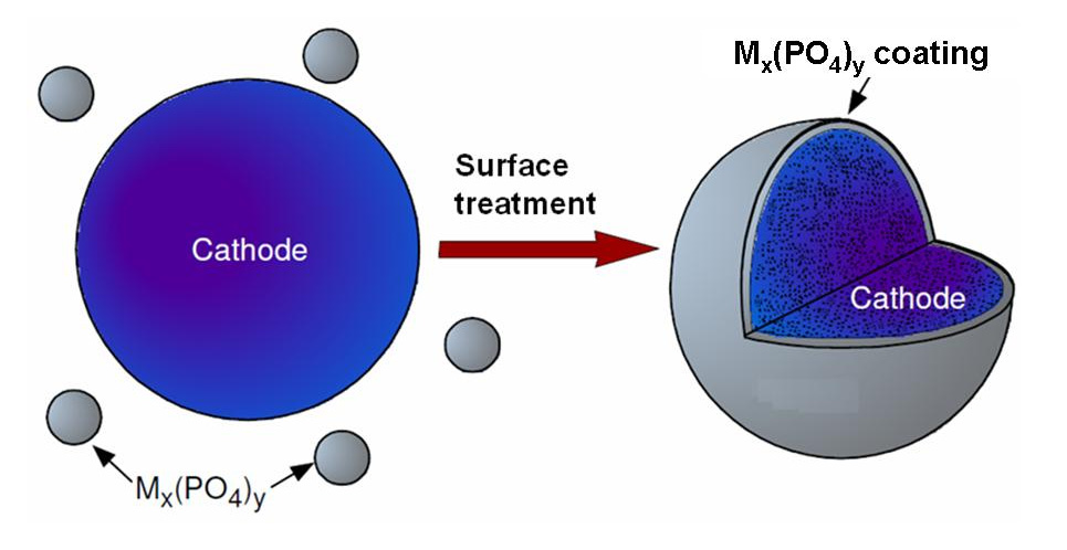
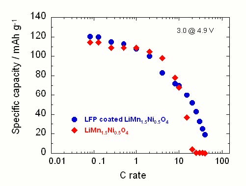
    [15] Liu D, Trottier J, Charest P, et al. (2012) Effect of nanoLiFePO4 coating on LiMn1.5Ni0.5O4 5-V cathode for lithium ion batteries. J Power Sources 204: 127–132.
    [16] 
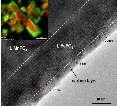
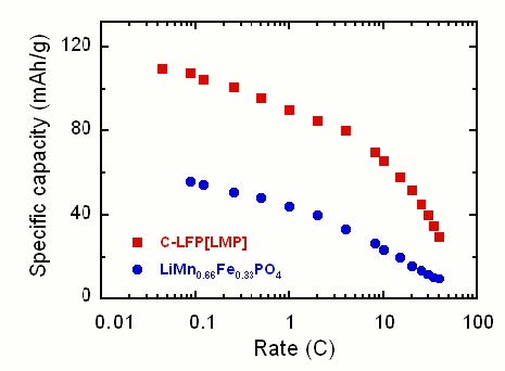
Zaghib K, Trudeau M, Guerfi A, et al. (2012) New advanced cathode material: LiMnPO4 encapsulated with LiFePO4. J Power Sources 204: 177–181. doi: 10.1016/j.jpowsour.2011.11.085
    [17] 
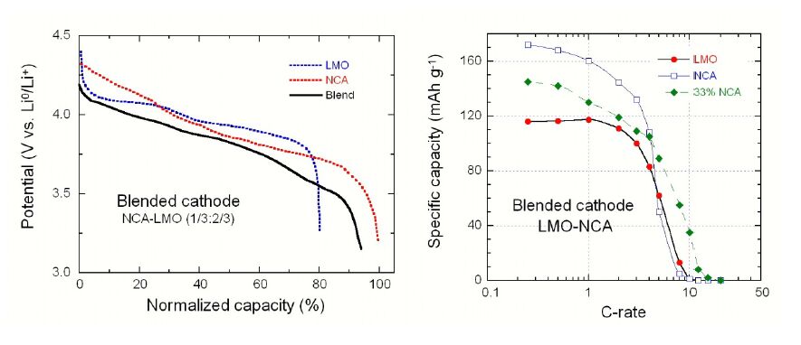
Chikkannanavar SB, Bernardi DM, Liu L (2014) A review of blended cathode materials for use in Li-ion batteries. J Power Sources 248: 91–100. doi: 10.1016/j.jpowsour.2013.09.052
    [18] Gao J, Manthiram A (2009) Eliminating the irreversible capacity loss of high capacity layered Li[Li0.2Ni0.13Mn0.54Co0.13]O2 cathode by blending with other lithium insertion hosts. J Power Sources 191: 644–647.
    [19] Tran HY, Täubert C, Fleischhammer M, et al. (2011) LiMn2O4 spinel/LiNi0.8Co0.15Al0.05O0.2 blends as cathode materials for lithium-ion batteries. J Electrochem Soc 158: A556–A561.
    [20] Luo W, Li X, Dahn JR (2010) Synthesis, characterization and thermal stability of Li[Ni1/3Mn1/3Co1/3-z(MnMg)z/2]O2. Chem Mater 22: 5065–5073. doi: 10.1021/cm1017163
    [21] 
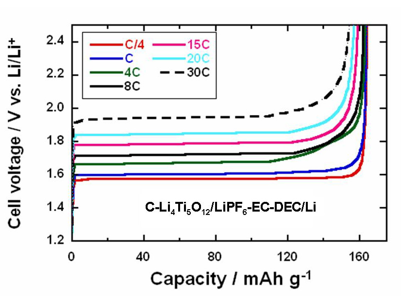
Ohzuku T, Ueda A, Yamamoto N (1995) Zero-strain insertion material of Li[Li1/3Ti5/3]O4 for rechargeable lithium cells. J Electrochem Soc 142: 1431–1435. doi: 10.1149/1.2048592
    [22] Zhu GN, Liu HJ, Zhuang JH, et al. (2011) Carbon-coated nano-sized Li4Ti5O12 Yong-Gang nanoporous micro-sphere as anode material for high-rate lithium-ion batteries. Energy Environ Sci 4: 4016–4022.
    [23] Wang YQ, Gu L, Guo YG, et al. (2012) Rutile-TiO2 nano-coating for a high-rate Li4Ti5O12 anode of a lithium-ion battery. J Am Chem Soc 134: 7874–7879. doi: 10.1021/ja301266w
    [24] Shen L, Li H, Uchaker E, et al. (2012) General strategy for designing core−shell nanostructured materials for high-power lithium ion batteries. Nano Lett 12: 5673–5678. doi: 10.1021/nl302854j
    [25] Choi JH, Ryu WH, Park K, et al. (2014) Multi-layer electrode with nano-Li4Ti5O12 aggregates sandwiched between carbon nanotube and graphene networks for high power Li-ion batteries. Sci Rep 4: 7334. doi: 10.1038/srep07334
    [26] Zaghib K, Dontigny M, Guerfi A, et al. (2012) An improved high-power battery with increased thermal operating range: C-LiFePO4//C-Li4Ti5O12. J Power Sources 216: 192–200. doi: 10.1016/j.jpowsour.2012.05.025
    [27] Jung HG, Myung ST, Yoon CS, et al. (2011) Microscale spherical carbon-coated Li4Ti5O12 as ultra-high power anode material for lithium batteries. Energy Environ Sci 4: 1345–1351. doi: 10.1039/c0ee00620c
    [28] Zaghib K, Dontigny M, Guerfi A, et al. (2012) An improved high-power battery with increased thermal operating range: C-LiFePO4//C-Li4Ti5O12. J Power Sources 216: 192–200. doi: 10.1016/j.jpowsour.2012.05.025
  • This article has been cited by:

    1. X. D. Chen, J. Wang, M. Z. Zhao, F. Zhao, Characterization and expression analysis of circadian clock genes in the diploid woodland strawberry Fragaria vesca, 2018, 62, 00063134, 451, 10.1007/s10535-018-0793-4
    2. Seok Joo Chae, Dae Wook Kim, Seunggyu Lee, Jae Kyoung Kim, Spatially coordinated collective phosphorylation filters spatiotemporal noises for precise circadian timekeeping, 2023, 26, 25890042, 106554, 10.1016/j.isci.2023.106554
  • Reader Comments
  • © 2016 the Author(s), licensee AIMS Press. This is an open access article distributed under the terms of the Creative Commons Attribution License (http://creativecommons.org/licenses/by/4.0)
通讯作者: 陈斌, bchen63@163.com
  • 1. 

    沈阳化工大学材料科学与工程学院 沈阳 110142

  1. 本站搜索
  2. 百度学术搜索
  3. 万方数据库搜索
  4. CNKI搜索

Metrics

Article views(10040) PDF downloads(1983) Cited by(8)

Article outline

Figures and Tables

Figures(13)

/

DownLoad:  Full-Size Img  PowerPoint
Return
Return

Catalog